Machine Learning Series (Part 36) : Why Logistic Regression Uses Log Loss Instead of MSE

Image Courtesy : ChatGPT

Good day readers! In the last blog we saw about the sigmoid function and the way to calculate the maximum likelihood of logistic regression. We all are very well aware of the cost function that we discussed during linear regression. The cost function plays the role of measuring out the error in the predictions of the model. Based on the error value, the weights of the model were adjusted to check if the cost function has decreased. Likewise, in logistic regression as well we calculate the cost function and proceed with gradient descent to update the weights and improvise the model. Today we are going to see all about the cost function of logistic regression. In the last blog, we all saw that the measure of how good the probability predicted by logistic regression can be seen through overall likelihood.

We had also seen a note that we can apply the log function to it.

And when we do so, by the log rule it turns into addition.

Now let us see how did we arrive at this:

Assume that there are 5 patients:

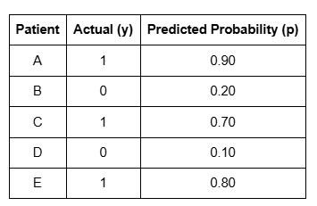
In the above set of records, we will now find the overall likelihood.

For patient A:

The actual (y) is 1 indicating the presence of heart disease. The predicted probability is 0.90

For patient B:

The actual (y) is 0 indicating the absence of heart disease. The predicted probability is 0.20, but whenever there is a negative prediction, we do (1-p). Because here, the negative prediction denotes the probability of not having a disease.

For patient C:

The actual (y) is 1 and the predicted probability is 0.70

For patient D:

The actual (y) is 0 which is the absence of heart disease and the predicted probability is 0.10. But the probability of not having a heart disease is 0.90

For patient E:

The actual (y) is 1 and the predicted probability is 0.80

The overall likelihood is:

If you notice the pattern, whenever the actual value is 1, we are considering the p value and whenever the actual value is 0, we are considering the (1-p) value.

Now how can we represent this scenario in a single equation?

If y = 1, then:

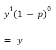
This is because

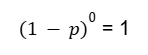
as anything power 0 is 1.

If y = 0 then:

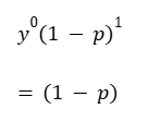
This gives us (1- p) as y⁰ is 1

The above two scenario of y=1 and y=0 can be easily represented in generic way as:

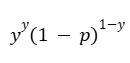
Now this is our final representation of the overall likelihood.

This has to be carried out for all the values. So we need to multiply likelihood for all the predictions.

When we do a summation of a set of values, we use the

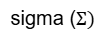
likewise when we do the product of a set of values, we use the

So the overall likelihood becomes:

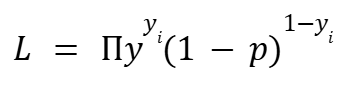
The i denotes the nth observation.

Now applying log to this as we had seen initially as well as in the previous blog gives:

From this we get:

Today we are going to see another logarithmic formula which is:

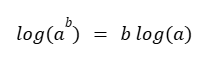
So the the equation becomes:

You might all wonder that the objective of this part is to cover the cost function. But why are we deep diving into the maximum likelihood right?

Don’t worry our next step is to find the cost function. Having derived the maximum likelihood, the cost function of logistic regression is just the negative of the above equation.

This is called log loss.

Here comes the greatest question, why are we just adding negative log to the maximum likelihood and how does this become the cost function of the logistic regression.

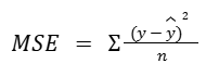
Because in linear regression, the cost function was the MSE which was the squared difference of the actual and the predicted value.

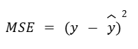
For example, if the actual value is 10 and the predicted value is 12

Then MSE is (10–12)².

As we had seen, if it deals with continuous value — like the house price prediction, then we can determine how erroneous the model was in case the actual price is 48 L and the predicted price is 50 L. Farther the prediction away from the actual value, higher is the error.

But in logistic regression, it is always either 1 (yes) or 0 (no). But if we do the same MSE to logistic regression, let’s say the actual value is 1 (having heart disease) and the model predicted 0.90, then the MSE is (1–0.90)²= 0.01. This difference is lower and tells that the prediction is good. Similarly, when we have the actual is 1 and the predicted is 0.40, the squared difference is 0.36 which tells that the error is high. When the actual is 1 and the prediction is 0.01, the squared difference is 0.98. This error conveys that there is a wide gap between the actual and the predicted.

But then why did we just multiply the maximum likelihood with -1 and call it log loss? It is because we wanted to minimize the error. We will see the reason very soon but before that let’s recollect the similar example that we saw earlier.

The actual house price is 100L but the model predicted as 95L, the error value is: (100–95)²= 25

In terms of logistic regression, consider two different model’s behaviour.

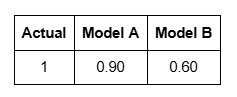
For model A, the error is 1–0.90 = 0.1 For model B, the error is 1–0.60 = 0.4

For the above two, the errors are corresponding to the model’s prediction. Consider two other models now:

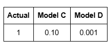
For model C, the error is 1–0.10 = 0.9 For model D, the error is 1–0.001 = 0.999

Model D is worse than model C, but did you see the error? The squared error increases, but it does not punish highly confident wrong predictions as aggressively as log loss.

Predicting 0.001 for an actual value of 1 (having heart disease) is very worse than predicting 0.1 right? That is why we find the likelihood to answer the question ‘How likely was the event that actually occurred? ’ The same if we apply it the negative log to it, we get

For model A, — log(0.95) = 0.051 For model B, -log(0.60) = 0.51 For model C, -log(0.10) = 2.3 For model D, -log(0.001) = 6.9

Now are you able to notice that the log loss is penalizing the model prediction that is not close to the actual value?

So instead of thinking like ‘How far is my prediction from the actual value?’ (as like in linear regression), researchers thought ‘How much probability did the model assign to the event that actually occurred? ’.

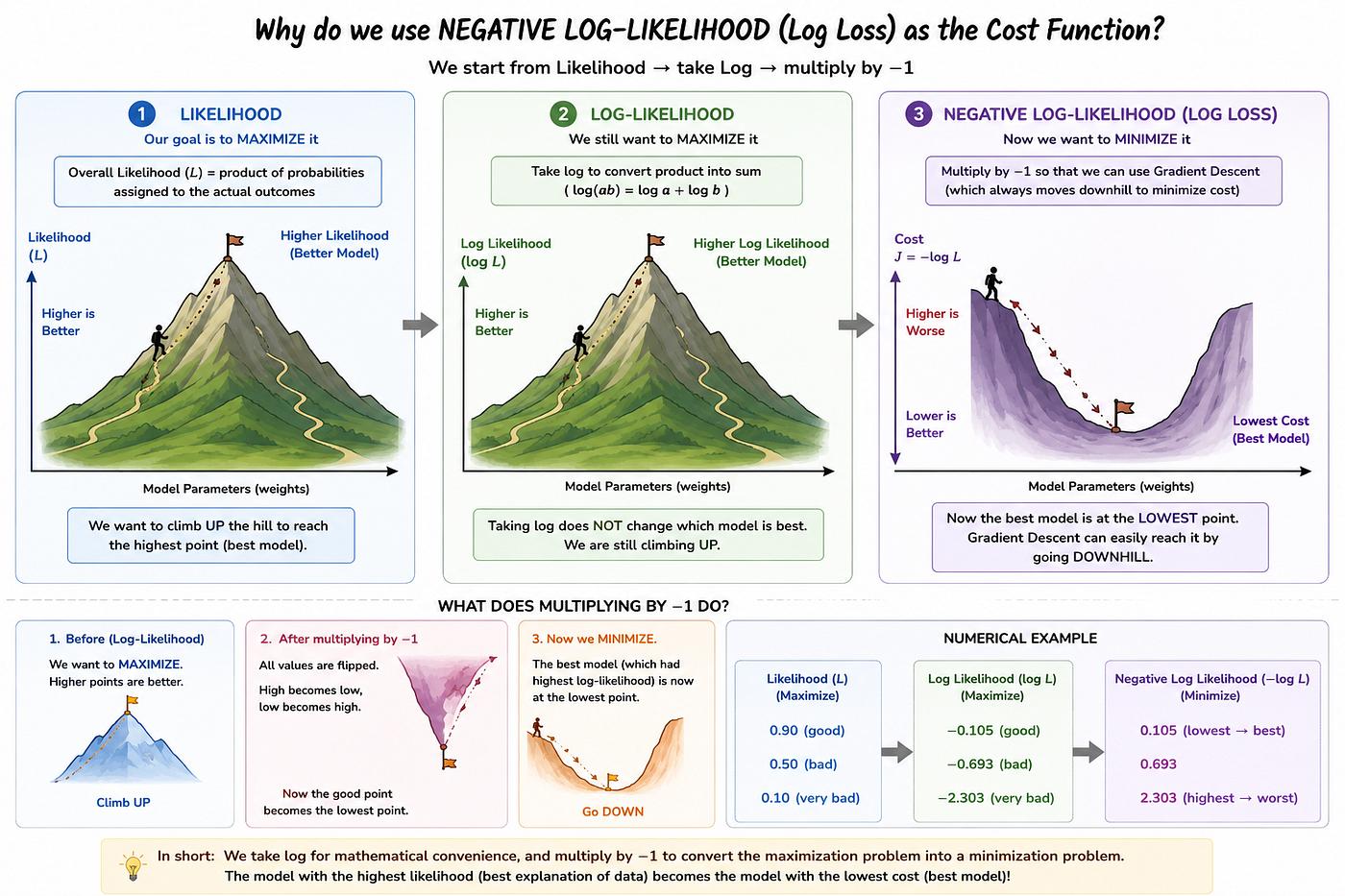
But why do we have the minus sign in the log loss is because gradient descent always chooses the opposite direction to the gradient (slope) of the loss to minimize the error. You can understand this by imagining our hill climbing example that we saw during our gradient descent blog where the hill’s surface is the loss and we have to move towards the lowest point. If our loss points to the higher surface, we need to move opposite to that. The minus sign changes our goal from finding the highest value to finding the lowest value. Since Gradient Descent works by minimizing a cost function, we simply multiply the log-likelihood by −1.

There is still another important reason why the MSE is not chosen for logistic regression.

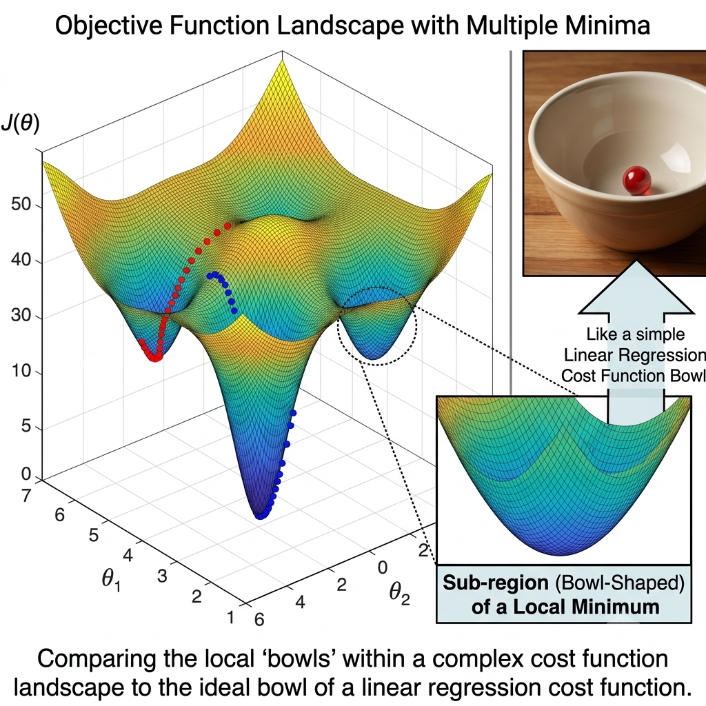
The actual problem lies in the shape of the cost function. When we were learning gradient descent, we saw that the cost function is kind of a mountainous terrain. There could be multiple local minima and a final global minimum. If we observe the minimum area, it is kind of a bowl. The following image illustrates this.

But if we consider the same MSE for the cost function instead of the log loss, it would appear like:

(actual — predicted)²

Here the predicted is the likelihood by the logistic regression model:

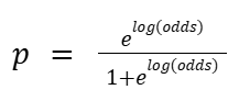
Note that in many cases, the

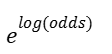
is represented by the alphabet z

So the notation becomes:

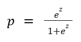
And they divide both the numerator and the denominator with e^z.

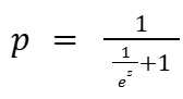
Now the

becomes e^-z. So the overall equation looks as:

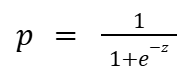
So now, if we substitute this in the actual minus predicted, the equation becomes as:

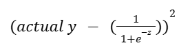
We all are very clear from the previous part that the prediction by the logistic regression which is basically the likelihood follows an S shaped curve (i.e. sigmoid shape). But in the linear regression, the MSE follows a bowl shaped loss surface, when the sigmoid shape is combined with the bowl shaped terrain , the loss surface becomes unsuitable to find the global minimum.

Here is an example surface for MSE:

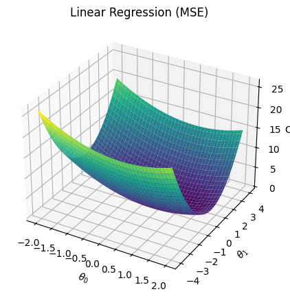
The MSE for logistic regression (incase the likelihood is applied in the actual minus predicted formula), the surface looks as:

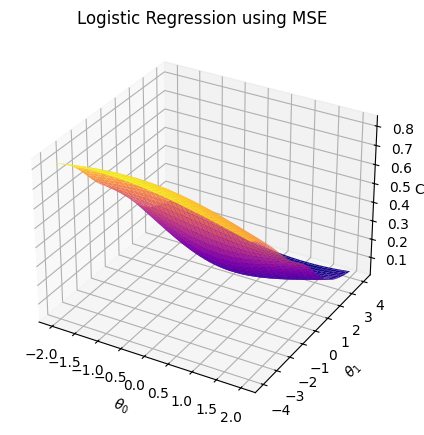
Could you see the difference? There is no clear global minimum in the loss surface. It becomes difficult to find the optimized parameters which is the core significance of gradient descent.

Conclusion:

In this blog, we understood why MSE is not suitable for logistic regression and how likelihood helps us measure the quality of a model’s predictions. By taking the negative log of the likelihood, we obtain a cost function that Gradient Descent can minimize efficiently. In the next part, we’ll see a quick implementation of logistic regression.