Knowledge Graph Construction and Querying with Deepseek-R1 7B vs Mistral 7B on Neo4j

Will Deepseek-R1 chain of thoughts approach generate meaningful graphs and lead to end of hallucinations? Not quite.

Photo by Irina Iriser on Unsplash

If you don’t have a Medium account, click here to access the full article.

Unless someone has been out on a camping trip deep in the forest with no outside contact, it is nearly impossible not to have heard about DeepSeek, a Chinese AI startup taking the world by storm. Their LLM Deepseek-R1 has almost become a household name even though it was just released a couple of weeks ago. Its release led to Nvidia to lose more than half a trillion dollars from its market value. The model has also been open-sourced, and in this short period, it had recorded over 1 million downloads just of its largest model on HuggingFace!

Deepseek-R1 is a Mixture of Experts model, trained with reinforcement learning. It is a huge model, 671 billion parameters in total, but only 37 billion active during inference. This startup company claimed that their model is on par with OpenAI o1, even though it was trained at a fraction of cost. In addition, they also created six more models simply by fine-tuning some other open-source LLMs, like Llama 3.1 and Qwen 2.5 with synthetic data generated with Deepseek-R1. These are termed distilled models, whereby a more powerful model trains a smaller model with synthetic data. Similar to the OpenAI o1 family of models, Deepseek-R1 is a reasoning model — instead of responding instantly like the traditional model, it has a thinking time, which aims to improve response.

In this article, we will explore how to adopt a Deepseek-R1 distilled model on a resource constrained machine for question-answering about local documents of a niche domain. To improve the performance in a niche domain, we will exploit the benefit of GraphRAG where we use the context from knowledge graphs constructed from these documents for improved response generation as well as to minimize hallucinations. For the knowledge graph construction, we will call upon LlamaIndex. The graphs themselves will be stored on Neo4j, a production-grade native graph database. To gauge how well Deepseek-R1 performs in this scenario, we will compare its graph construction and response generation aspects against the trusty Mistral 7B.

Let’s get started!

1.0 Technology Stack and Environment Setup

As the focus of application is for a resource-constrained setup, this work was undertaken on a MacBook Air M1 with 8GB RAM running MacOS Ventura. The version of Python used was 3.11.5.

Firstly, let’s create a virtual environment to manage this project. To create and activate the environment, run the followings:

python3.11 -m venv kg_qa
source kg_qa/bin/activate

The framework for our system uses LlamaIndex, as it readily provides tools for data ingestion, indexing and querying. It also has module PropertyGraphIndex, which handles automated knowledge graph construction from unstructured text with the help of LLM as well as facilitates entity-based querying.

To facilitate Neo4j as a graph store for our knowledge graphs, we will adopt module Neo4jPropertyGraphStore. In addition, Python driver for Neo4j, named neo4j, is also needed. If you are looking for a primer on this graph database, its setup, its web UI as well as its query language, Cypher, feel free to check out this earlier article:

[embed]Local LLM Generated Knowledge Graphs Powered by a Local Neo4j Graph Database How does its generation performance compare to a SimpleGraphStore storage?ai.gopubby.com

To allow support for a local LLM, we will use the amazing llama-cpp-python library with Metal support. Figure 1 shows the list of Deepseek-R1 distilled model as shown on its HuggingFace repo along with the base models used for fine-tuning. For a resource constrained setup, we will adopt the quantized models made available on unsloth HuggingFace repo, especially Deepseek-R1 7B Q2_K model.

Fig. 1. List of DeepSeek-R1 distilled models from HuggingFace

For our performance comparison, the Deepseek-R1 2-bit model will be pitted against 2-bit Mistral 7B Instruct v0.3 Q2_K.

Let’s take a quick look at the implemention.

2.0 System Implementation

This design is based on the same approach presented in the previous work. Firstly, let’s import all the required modules, as per below:

from llama_index.core import (
    PropertyGraphIndex,
    SimpleDirectoryReader,
    StorageContext,
    Settings,
)
from llama_index.llms.llama_cpp import LlamaCPP   # version 0.4.0
from llama_index.embeddings.huggingface import HuggingFaceEmbedding
from llama_index.graph_stores.neo4j import Neo4jPropertyGraphStore

Instantiate a LlamaCPP object to load the required model from local directory ./models as well as the selected embeddings model. To allow this LLM to be used globally by LlamaIndex modules, assign class Settings property llm to this LLM instance and the embeddings model. The following code extract summarizes these steps:

llm = LlamaCPP(
    model_path='./models/DeepSeek-R1-Distill-Qwen-7B-Q2_K.gguf',
    temperature=0.6,
    max_new_tokens=2000,
    context_window=4096,
    model_kwargs={"n_gpu_layers": 1},
    verbose=False                                                                                                                                                                                              
)
embed_model = HuggingFaceEmbedding()
Settings.llm = llm
Settings.embed_model = embed_model
Settings.chunk_size = 512

Unlike a smaller model temperature of 0.1 used for Mistral 7B, we will use 0.6 for DeepSeek-R1 7B as recommended by DeepSeek authors. To setup a graph store backed by our Neo4j database, let’s instantiating a Neo4jPropertyGraphStore object using default credentials and database name, as shown next:

url = "bolt://localhost:7687"
username = "neo4j"
password = "password"
database = "neo4j"

graph_store = Neo4jPropertyGraphStore(
    username=username,
    password=password,
    url=url,
    database=database,
)

With this graph_store, lets proceed to create a StorageContext instance. To load documents, we will use SimpleDirectoryReader to read from directory ./pdf/. To construct knowledge graphs from these documents, we use method PropertyGraphIndex.from_documents.

gstorage_context = StorageContext.from_defaults(graph_store=graph_store)                                                                                                                                       
documents = SimpleDirectoryReader("./pdf/").load_data()
kg_index = PropertyGraphIndex.from_documents(
    documents,
    storage_context=gstorage_context,
    max_triplets_per_chunk=10,
    include_embeddings=True,
    property_graph_store=graph_store,
)

Once graphs are constructed, they are automatically saved to the Neo4j database by PropertyGraphIndex. At this juncture, the graphs would be available for querying. Create a query engine off the graph index. Using the recommended Deepseek-R1 prompt where only user prompt is suggested without a separate system prompt, the template looks like <｜User｜>{query}<｜Assistant｜>:

kg_keyword_query_engine = kg_index.as_query_engine(
    include_text=True,
    similarity_top_k=2,
)
query = 'When should simplified routing be used on SteelHeads?'
response = kg_keyword_query_engine.query(f'<｜User｜>{query}<｜Assistant｜>')

With just a few lines of code, the basic code is ready for us to take it for a spin.

3.0 Performance Comparison

3.1 Knowledge Graph Construction

Before we can run the above system, Neo4j DBMS needs to started first and be available on the localhost. For this experimentation, we will adopt two separate knowledge-base (KB) articles on SteelHead, a technology related to WAN app acceleration, to represent our niche domain. The first KB talks about a feature called simplified routing, which helps the device to automatically learn and forward network packets to the appropriate next hop. The second KB discusses how to enable the HTTP/2.0 acceleration feature on the SteelHeads. For this test across both models, the graph construction prompt used was the LlamaIndex default.

Figure 2 depicts the generated graphs when the first KB was ingested with the help of Deepseek-R1. The graph on the right that includes entity “Simplified routing” seems to have captured the embedded knowledge mostly well, except for the relationship “is using” to entity “Static routes”. This SteelHead feature does not directly rely on the presence static routes.

Fig. 2. Knowledge graphs generated by Deepseek-R1 for KB #1. Image by author

For comparison, Fig. 3 shows the graphs generated with the help of Mistral 7B. It is immediately evident here that the Mistral graphs encoded a lot lesser details, although it did capture the high level mechanics of the simplified routing feature.

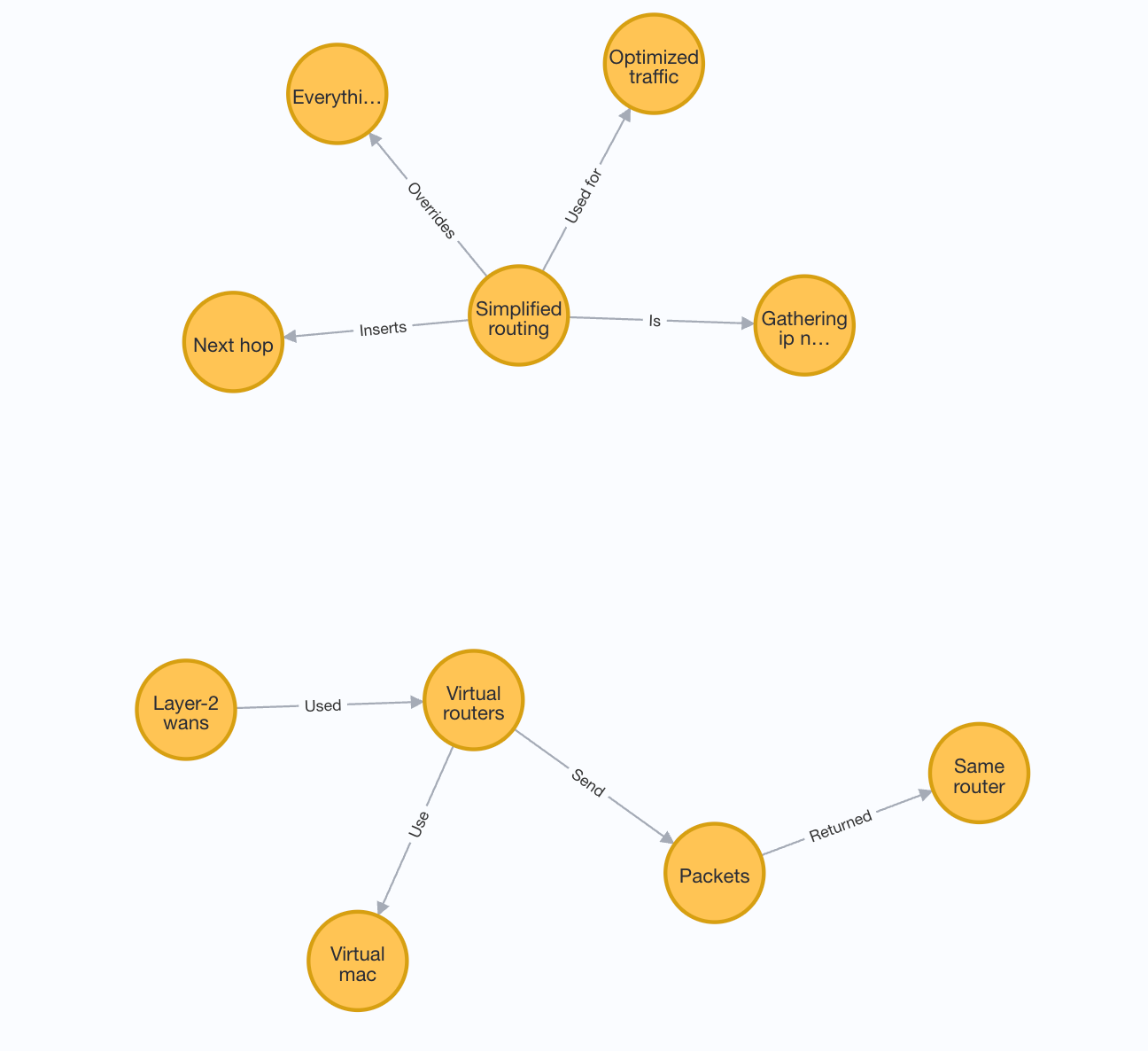
Fig. 3. Knowledge graphs generated by Mistral for KB #1. Image by author

For the second test, we reset the Neo4j database first and then undertake graph construction against KB #2, which talks about enabling HTTP/2.0 acceleration. Figure 4 depicts the knowledge graphs generated by Deepseek-R1 off this document. There are quite a few questionable entities and relationships generated here such as “1.2” and “2.0” for the former, and “Protocol” and “Http/2.0” for the latter. This encoding curiously doesn’t capture its knowledge.

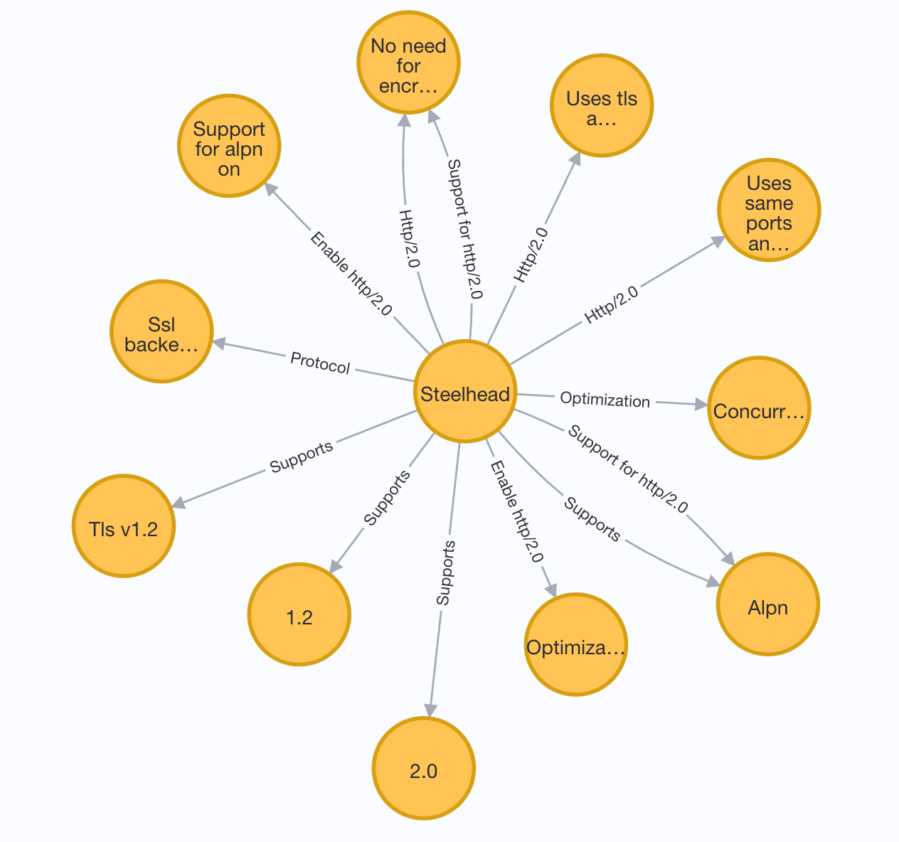
Fig. 4. Knowledge graphs generated by Deepseek-R1 for KB #2. Image by author

In contrast, Fig. 5 shows the resulting graphs when ingested with Mistral 7B. Similar to the previous KB ingestion, these Mistral graphs are again a lot simpler than Deepseek-R1’s. These graphs also appear to encode very limited details off this second KB.

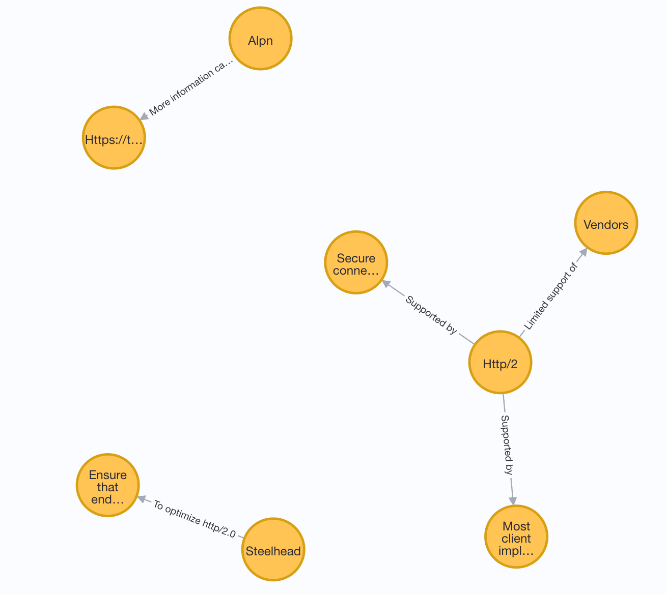
Fig. 5. Knowledge graphs generated by Mistral for KB #2. Image by author

Comparing the graphs constructed by both models across the two KBs, there is no clear winner here. Deepseek-R1 excelled when ingesting KB #1, but it did not fare as well against KB #2. Mistral 7B generated fairly simplistic graphs for both documents, but did not capture the nuances involved with those features.

Let’s now explore their querying performance across the two KBs.

3.2 Response Generation

The following is our the first prompt to gauge the models’ querying performance related to KB #1.

When should simplified routing be used on SteelHeads?

Let’s now take a look at Deepseek-R1’s performance against this query. The following output captures its full response.

<think>
Okay, so I need to figure out when to use simplified routing on a SteelHead appliance. I'm not too familiar with SteelHead, but I remember it's related to networking, probably for routers or firewalls. Simplified routing, from what I recall, is a feature that simplifies the routing process for the device, making it more efficient or easier to manage.

Looking at the context provided, there are several points mentioned. First, it says that simplified routing is gathering IP addresses to their MAC addresses. That means when the device receives a packet, it maps the IP address to a MAC address to determine where the traffic should go. This is important because IP addresses are addressable at the IP level, but devices typically communicate through MAC addresses at the MAC layer.

Another point mentions that simplified routing is responsible for the destination IP and MAC address. So, when the device sends out a packet, it uses this information to route it correctly. Simplified routing is using the destination IP and MAC address to determine the next hop.

The context also talks about when it's responsible for the same address. That might be referring to when the source or destination IP is the same as the MAC address, which can happen when dealing with multi-homed networks or when a router has multiple interfaces.

The context further explains that simplified routing is using the MAC address to send out traffic, which is important because it helps the device know which interface to send the packet out and which to receive it on. This is crucial for layer-2 WANs, which are large networks that require efficient routing across multiple locations.

The context also mentions that if the default gateway doesn't have the right ACLs (Access Control Lists), it might drop traffic that should have gone through another router. So, the user has to add static routes to direct traffic through the other router. But the solution provided by simplified routing is to avoid using those static routes by using the MAC address when sending out packets.

Another important point is about the destination being a new TCP connection. Simplified routing allows the device to insert the next hop interface when sending out a packet, overriding other routing steps if there's no mapping. This is useful because in some cases, especially in complex networks, the default routing might not be sufficient, and the device can dynamically insert the correct next hop based on the MAC address.

The context also warns about when not to use simplified routing. It says that simplified routing can't be used with broadcast support, WCCP (Wide Area Connection Point, which is related to IEEE 802.1Q VLANs), or PBR (Polymorphic Packet Reordering, used in some load balancers). So, if the environment requires those features, simplified routing isn't suitable.

Lastly, the context explains that simplified routing is best for scenarios where the network is being optimized through the SteelHead. It's a simplified version of the routing process, making it easier to manage and less resource-intensive. It's not for every situation, though; it's specifically for certain network topologies and scenarios.

Putting this together, simplified routing on a SteelHead should be used when you have a network that's being optimized, specifically in scenarios where you have multiple subnets or multiple VLANs that need to be optimized. It's especially useful in layer-2 WAN deployments where the network is large and complex. It's best used when you can define one router as the default gateway and have other routes configured via static routes or additional static routes to direct traffic through other routers. This avoids the need for complicated ACLs that might be required without simplified routing.

I think that covers the main points. It's a bit complex, but I think I have a good grasp now.
</think>

Simplified routing on a SteelHead appliance should be used in the following scenarios:

1. **Network Optimization**: When optimizing a network topology, especially in environments with multiple subnets or VLANs that need optimization.

2. **Layer-2 WANs**: For large networks requiring efficient routing across multiple locations.

3. **Multiple Subnets/VLANs**: When multiple subnets or VLANs need to be optimized through the SteelHead.

4. **No Need for Complicated ACLs**: When the default gateway doesn't require complex ACLs to direct traffic through other routers.

5. **Destination IP Handling**: When dealing with destinations that are the same address, as simplified routing handles this efficiently.

6. **Dynamic Next Hop Insertion**: When the destination is a new TCP connection, as simplified routing allows the device to insert the correct next hop interface dynamically.

7. **Avoid broadcast support, WCCP, or PBR**: When the environment doesn't require these features, as simplified routing can't be used with them.

In summary, use simplified routing for optimized large networks, especially in scenarios involving multiple subnets or VLANs, without requiring complex ACLs for traffic routing. It's ideal for scenarios where dynamic next hop insertion is needed and where broadcast support, VLANs, or PBR isn't required.

The key behavior of a reasoning model is at fully display here. It has the <think> section which captures the model’s chain of thoughts. Here, Deepseek-R1 clearly admits its lack of familiarity with this domain: I’m not too familiar with SteelHead. Also, it immediately calls upon the context that was provided, and explores each point one at a time. This thought process was spot on. Near the end of the <think> section, the model notes: I think I have a good grasp now. The actual response followed thereafter but it too was very verbose. Five of seven points were perfect. However, the model hallucinated with points #5 and #6.

Let’s now take a look at Mistral 7B’s response for the same prompt:

Simplified routing should be used on SteelHeads when traffic is redirected back through a SteelHead and the user does not want to add static routes for the other router. Simplified routing gathers the IP to next hop MAC address mapping from each packet it receives to use in addressing its own traffic, which overrides everything else. This allows optimized traffic to be sent directly to the next hop without the need for static routes.

This response describes what is simplified routing precisely and concisely suggests when this feature should be used. However, this response does not capture the nuances of its application, which was present in Deepseek-R1’s response. For this query, the winner is Mistral 7B, as it did not hallucinate.

Table 1 summarizes all three questions and responses as well as the response times for both models about KB #1. For all Deepseek-R1’s responses, it is shown without the <think> section as well as the response had to be snipped to limit space. For each query, the best response is highlighted in green, and the least response time (in seconds) is shown in bold. In a surprising development, Mistral 7B had concise and accurate direct answers to all three queries. Deepseek-R1 responses were nuanced and captured different scenario at length, but also included hallucinated facts. Deepseek-R1 response to Q3 assumed SteelHead is a load balancing solution, when in fact it is an app acceleration technology. In addition, Deepseek-R1’s response were up to 3.5x slower than Mistral 7B. Even its graph construction time was more than 6x slower.

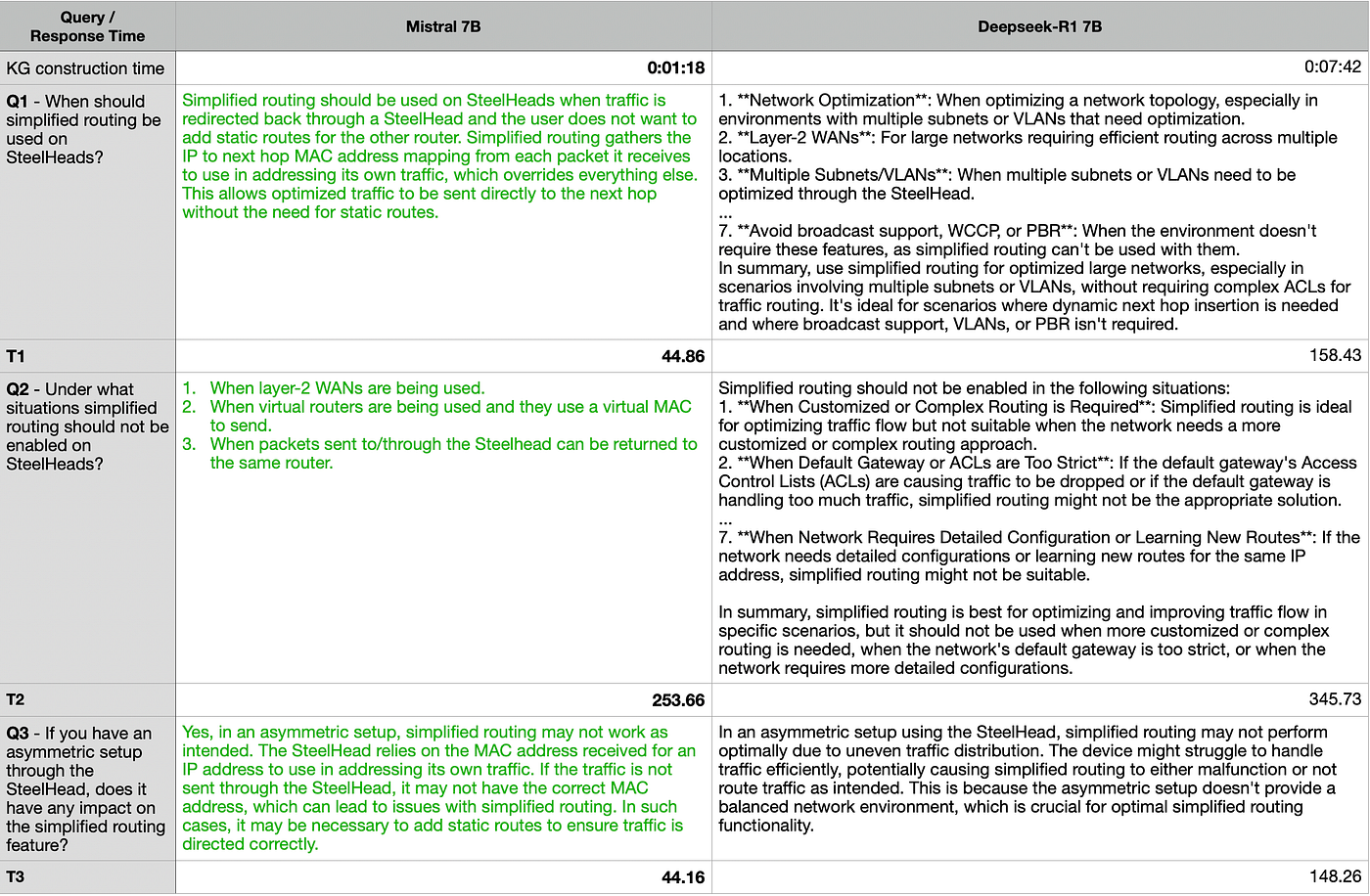
Table 1. Response generation performance against KB #1.

Table 2 captures response generation performance of both models when queried about KB #2. During this test, Deepseek-R1 responses were a lot left to be desired for Q2 and Q3. For Q2, although its chain of thoughts seemed reasonable (not shown), Deepseek-R1 provided an invalid command. This lack of performance directly related to the unexpected knowledge graphs that were produced by this model as shown earlier in Fig. 4. In addition, Deepseek-R1 response time up to 7.7x slower than Mistral 7B.

Table 2. Response generation performance against KB #2.

Based on these observations and the limited test scenarios explored here, Deepseek-R1 appears to face some challenges around knowledge graph construction with its inconsistent behavior against different contents. However, it will be interesting to see if this observation generalizes to its lesser lossy versions.

4.0 Concluding Remarks

The use of LLMs is expanding to niche domains, where the models may not have seen during their pretraining. Using context from knowledge graphs off such content has been shown to perform well in such scenarios. They capture the semantic relationship of entities. With the market-disrupting entry of Deepseek-R1, it is only apt for us to exercise this model for graph construction and querying.

In this article, we developed a simple QA system to query local documents in a resource constrained setup. We pitted a 2-bit quantized Deepseek-R1 7B distilled model against a similar Mistral 7B configuration using a Neo4j graph database as its backend. Two knowledge-base documents of a niche domain were independently ingested. Deepseek-R1 successfully encoded one document nearly all of its embedded knowledge, but it didn’t fare as well with the second document. On the contrary, Mistral 7B was a lot more simplistic in its graph construction, capturing just the main facts rather accurately.

When it came to querying performance, a gulf opened between the models. Deepseek-R1 provided nuanced detail responses but along with hallucinated facts to most questions! Mistral 7B was spot on with its concise but simplistic responses. In addition, Mistral 7B was able to respond up to 7.7x quicker. If you are contemplating the adoption Deepseek-R1 for querying your local documents, there are some challenges to overcome not the least its response time. Will this pattern of behavior be retained for higher-precision models, such as 4-bit models? This will be an interesting further work to take home for a more resourced setup. 😅

Thanks for reading!