Resample & Rebalance: Your Second Practical Guide to Backtesting.

source of the image

This is the second part of a guide consists of three parts, in each part you’ll discover how to do basic backtesting for avoid losing your money, in this one we will talk about doing a simple strategy used by Robert Carver and it’s issues , in the last one we will do take a simulation of 60/40 portfolio and using two different ETFs, and a Bonus part.

Take a seat please, and brew your black gold for yourself, and start reading the blog and the opening a clean notebook.

Simple Moving Average Crossover Strategy

1. Compute 20-day and 50-day Moving Averages for SPY
2. Generate buy/sell signals when short MA crosses above/below long MA.
3. Backtest the Crossover Strategy.
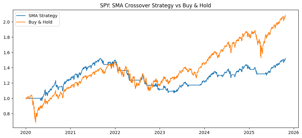
4. Calculate and Plot strategy Equity Curve vs. Buy-and-Hold.
5. Add Basic Transaction Costs.
6. Compute Number of Trades per Year.
7. Testing Performance using Resampled Monthly Data Instead of Daily.
8. Parametrize MA Windows and Optimize for Best Sharpe Ratio In-Sample.
9. Compare Results using SMA (simple) vs. EMA (exponential moving average).
10. Apply the strategy to another ETF (e.g., QQQ or AGG).

The goal is straightforward: take SPY, calculate two moving averages, turn them into trading decisions, and measure what happens with costs and variations included, sounds like a kid game.

1. Compute 20-day and 50-day Moving Averages for SPY

import pandas as pd
import numpy as np
import matplotlib.pyplot as plt
from alpaca.data.historical import StockHistoricalDataClient
from alpaca.data.requests import StockBarsRequest
from alpaca.data.timeframe import TimeFrame
from datetime import datetime

client = StockHistoricalDataClient(ALPACA_API_KEY, ALPACA_API_SECRET)

# Helper: Fetch daily bars
def fetch_daily_data(ticker, start="2020-01-01", end=None):
    if end is None:
        end = datetime.today().strftime("%Y-%m-%d")
    request = StockBarsRequest(
        symbol_or_symbols=ticker,
        timeframe=TimeFrame.Day,
        start=pd.Timestamp(start, tz='America/New_York'),
        end=pd.Timestamp(end, tz='America/New_York')
    )
    bars = client.get_stock_bars(request).df
    if isinstance(bars.index, pd.MultiIndex):
        bars = bars.xs(ticker, level=0)
    bars = bars.reset_index()
    bars.set_index("timestamp", inplace=True)
    return bars

spy_daily = fetch_daily_data("SPY")

spy_daily['sma20'] = spy_daily['close'].rolling(20).mean()
spy_daily['sma50'] = spy_daily['close'].rolling(50).mean()
spy_daily[20:60]

open      high       low    close       volume  \
timestamp                                                                       
2020-01-31 05:00:00+00:00  327.0000  327.1700  320.7300  321.750  116500962.0   
2020-02-03 05:00:00+00:00  323.3500  326.1600  323.2200  324.120   71170107.0   
2020-02-04 05:00:00+00:00  328.0700  330.0100  327.7200  329.060   64065469.0   
2020-02-05 05:00:00+00:00  332.2700  333.0900  330.6700  332.840   67402342.0   
2020-02-06 05:00:00+00:00  333.9100  334.1900  332.8000  333.930   51626082.0   
2020-02-07 05:00:00+00:00  332.8200  333.9941  331.6000  332.240   65101736.0   
2020-02-10 05:00:00+00:00  331.2300  334.7500  331.1900  334.750   43576992.0   
2020-02-11 05:00:00+00:00  336.1600  337.0200  334.6840  335.270   55707407.0   
2020-02-12 05:00:00+00:00  336.8300  337.6500  336.4300  337.440   44997697.0   
2020-02-13 05:00:00+00:00  335.8621  338.1200  335.5600  337.170   55382831.0   
2020-02-14 05:00:00+00:00  337.5100  337.7300  336.2000  337.600   65012969.0   
2020-02-18 05:00:00+00:00  336.5100  337.6677  335.2100  336.730   58482788.0   
2020-02-19 05:00:00+00:00  337.7900  339.0800  337.4800  338.320   49804453.0   
2020-02-20 05:00:00+00:00  337.7423  338.6400  333.6817  336.990   74976767.0   
2020-02-21 05:00:00+00:00  335.4700  335.8100  332.5800  333.450  115144054.0   
2020-02-24 05:00:00+00:00  323.1400  333.5623  321.2400  322.420  163655089.0   
2020-02-25 05:00:00+00:00  323.9400  324.6100  311.6900  312.590  223245173.0   
2020-02-26 05:00:00+00:00  314.1800  318.1100  310.7000  311.610  198369131.0   
2020-02-27 05:00:00+00:00  305.4600  311.5637  297.5100  297.700  288117319.0   
2020-02-28 05:00:00+00:00  288.7000  297.8920  285.5400  296.240  392482615.0   
2020-03-02 05:00:00+00:00  298.2100  309.1600  294.4600  308.900  241275739.0   
2020-03-03 05:00:00+00:00  309.5000  313.8400  297.5700  300.320  305243992.0   
2020-03-04 05:00:00+00:00  306.1200  313.1000  303.3300  313.050  178853859.0   
2020-03-05 05:00:00+00:00  304.9800  308.4700  300.0100  302.510  188896911.0   
2020-03-06 05:00:00+00:00  293.1500  298.7800  290.2300  297.430  231042459.0   
2020-03-09 04:00:00+00:00  275.3000  284.1900  273.4500  276.320  312908288.0   
2020-03-10 04:00:00+00:00  284.6400  288.5200  273.5000  288.410  278857139.0   
2020-03-11 04:00:00+00:00  280.7000  281.9400  270.8800  274.250  258486370.0   
2020-03-12 04:00:00+00:00  256.0000  266.6600  247.6800  255.240  394824960.0   
2020-03-13 04:00:00+00:00  263.0900  271.4754  248.5237  270.200  328921935.0   
2020-03-16 04:00:00+00:00  241.1800  256.9000  237.3600  241.065  300815897.0   
2020-03-17 04:00:00+00:00  245.0400  256.1700  237.0700  254.190  265602534.0   
2020-03-18 04:00:00+00:00  236.2500  248.3700  228.0200  235.690  329737404.0   
2020-03-19 04:00:00+00:00  239.2500  247.3800  232.2200  240.550  292164236.0   
2020-03-20 04:00:00+00:00  242.5300  244.4700  228.5000  229.400  346965271.0   
2020-03-23 04:00:00+00:00  228.1900  229.6833  218.2600  222.680  328483538.0   
2020-03-24 04:00:00+00:00  234.4200  244.1000  233.8000  242.000  238855181.0   
2020-03-25 04:00:00+00:00  244.8700  256.3500  239.7500  246.790  301441274.0   
2020-03-26 04:00:00+00:00  249.5200  262.8000  249.0500  260.930  260651432.0   
2020-03-27 04:00:00+00:00  253.2700  260.8100  251.0500  254.000  225910512.0   

                           trade_count        vwap      sma20     sma50  
timestamp                                                                
2020-01-31 05:00:00+00:00     653950.0  322.929426  327.07500       NaN  
2020-02-03 05:00:00+00:00     368446.0  324.650151  327.15950       NaN  
2020-02-04 05:00:00+00:00     312753.0  329.166476  327.42600       NaN  
2020-02-05 05:00:00+00:00     352029.0  332.080961  327.93100       NaN  
2020-02-06 05:00:00+00:00     249696.0  333.719271  328.40650       NaN  
2020-02-07 05:00:00+00:00     299477.0  332.520910  328.68900       NaN  
2020-02-10 05:00:00+00:00     217772.0  333.450623  329.14450       NaN  
2020-02-11 05:00:00+00:00     268292.0  335.908311  329.51200       NaN  
2020-02-12 05:00:00+00:00     230201.0  337.059081  330.01300       NaN  
2020-02-13 05:00:00+00:00     287289.0  337.062706  330.46350       NaN  
2020-02-14 05:00:00+00:00     251609.0  337.051582  330.80050       NaN  
2020-02-18 05:00:00+00:00     286928.0  336.417747  331.03650       NaN  
2020-02-19 05:00:00+00:00     221056.0  338.447732  331.38800       NaN  
2020-02-20 05:00:00+00:00     431814.0  336.210263  331.67000       NaN  
2020-02-21 05:00:00+00:00     487163.0  333.722906  331.75250       NaN  
2020-02-24 05:00:00+00:00     872755.0  323.659244  331.43550       NaN  
2020-02-25 05:00:00+00:00    1448758.0  316.242191  330.88950       NaN  
2020-02-26 05:00:00+00:00    1374136.0  313.802163  330.12600       NaN  
2020-02-27 05:00:00+00:00    2154932.0  304.059447  328.68000       NaN  
2020-02-28 05:00:00+00:00    2685904.0  290.847617  327.11100       NaN  
2020-03-02 05:00:00+00:00    1763456.0  301.687408  326.46850       NaN  
2020-03-03 05:00:00+00:00    2844651.0  304.575142  325.27850       NaN  
2020-03-04 05:00:00+00:00    1261953.0  308.177865  324.47800       NaN  
2020-03-05 05:00:00+00:00    1265055.0  303.693158  322.96150       NaN  
2020-03-06 05:00:00+00:00    1641498.0  294.587353  321.13650       NaN  
2020-03-09 04:00:00+00:00    2577868.0  278.354295  318.34050       NaN  
2020-03-10 04:00:00+00:00    2516870.0  281.195869  316.02350       NaN  
2020-03-11 04:00:00+00:00    2152463.0  276.177671  312.97250       NaN  
2020-03-12 04:00:00+00:00    3709929.0  254.820022  308.86250       NaN  
2020-03-13 04:00:00+00:00    2669400.0  258.352780  305.51400  319.4694  
2020-03-16 04:00:00+00:00    2147760.0  246.753505  300.68725  317.7933  
2020-03-17 04:00:00+00:00    2175118.0  248.250670  296.56025  316.4285  
2020-03-18 04:00:00+00:00    2874735.0  236.712854  291.42875  314.6677  
2020-03-19 04:00:00+00:00    2855927.0  241.590533  286.60675  313.0239  
2020-03-20 04:00:00+00:00    2924219.0  236.368926  281.40425  311.1235  
2020-03-23 04:00:00+00:00    2848122.0  223.591385  276.41725  309.0453  
2020-03-24 04:00:00+00:00    1625798.0  239.148951  272.88775  307.3725  
2020-03-25 04:00:00+00:00    2166623.0  248.953723  269.64675  305.7499  
2020-03-26 04:00:00+00:00    1886244.0  257.188041  267.80825  304.4201  
2020-03-27 04:00:00+00:00    1671020.0  254.709711  265.69625  302.9369  

We start with daily closing prices in spy_daily['close']. A 20-day rolling mean reacts quickly. A 50-day mean moves slower. Both create new columns without changing the rest of your data. Two things to know: The first 19 and 49 rows will show NaN because there isn’t enough history yet. That’s normal. And use adjusted closes if your data have it, so stock splits and dividends don’t mess up your signals later.

2. Generate buy/sell Signals When Short MA Crosses above/below Long MA.

spy_daily['signal'] = 0
spy_daily.loc[spy_daily['sma20'] > spy_daily['sma50'], 'signal'] = 1  # Long only
spy_daily['position'] = spy_daily['signal'].shift(1).fillna(0)

 open      high      low   close      volume  \
timestamp                                                                  
2020-01-02 05:00:00+00:00  323.54  324.8900  322.530  324.87  60187033.0   
2020-01-03 05:00:00+00:00  321.16  323.6400  321.100  322.43  80319689.0   
2020-01-06 05:00:00+00:00  320.49  323.7300  320.360  323.73  56672077.0   
2020-01-07 05:00:00+00:00  323.02  323.5400  322.240  322.74  43646563.0   
2020-01-08 05:00:00+00:00  322.94  325.7800  322.670  324.42  69691471.0   
...                           ...       ...      ...     ...         ...   
2025-10-20 04:00:00+00:00  667.32  672.2100  667.270  671.30  60492650.0   
2025-10-21 04:00:00+00:00  671.44  672.9900  669.981  671.29  56248835.0   
2025-10-22 04:00:00+00:00  672.00  672.0000  663.300  667.80  80564006.0   
2025-10-23 04:00:00+00:00  668.12  672.7101  667.800  671.76  65604461.0   
2025-10-24 04:00:00+00:00  676.46  678.4700  675.650  677.25  74356527.0   

                           trade_count        vwap     sma20     sma50  \
timestamp                                                                
2020-01-02 05:00:00+00:00     304886.0  323.680084       NaN       NaN   
2020-01-03 05:00:00+00:00     358026.0  322.732865       NaN       NaN   
2020-01-06 05:00:00+00:00     255769.0  322.602237       NaN       NaN   
2020-01-07 05:00:00+00:00     226060.0  322.918261       NaN       NaN   
2020-01-08 05:00:00+00:00     340005.0  324.553163       NaN       NaN   
...                                ...         ...       ...       ...   
2025-10-20 04:00:00+00:00     858129.0  670.723645  665.2855  655.3516   
2025-10-21 04:00:00+00:00     831016.0  671.751723  665.6895  656.0590   
2025-10-22 04:00:00+00:00     963659.0  667.586309  666.0245  656.5612   
2025-10-23 04:00:00+00:00     767072.0  670.893450  666.7100  657.0986   
2025-10-24 04:00:00+00:00     762628.0  677.528460  667.4815  657.7446   

                           signal  position  
timestamp                                    
2020-01-02 05:00:00+00:00       0       0.0  
2020-01-03 05:00:00+00:00       0       0.0  
2020-01-06 05:00:00+00:00       0       0.0  
2020-01-07 05:00:00+00:00       0       0.0  
2020-01-08 05:00:00+00:00       0       0.0  
...                           ...       ...  
2025-10-20 04:00:00+00:00       1       1.0  
2025-10-21 04:00:00+00:00       1       1.0  
2025-10-22 04:00:00+00:00       1       1.0  
2025-10-23 04:00:00+00:00       1       1.0  
2025-10-24 04:00:00+00:00       1       1.0  

[1462 rows x 11 columns]

Here we turn the moving average comparison into a binary decision. Signal equals 1 when the fast line sits above the slow line, otherwise 0. The important part is shift(1). You learn about a crossover at today's close but can only trade the next day. Shifting enforces this discipline. fillna(0) means before the first signal exists, you're flat. This one line prevents look-ahead bias and separates honest backtests from fantasy.

3. Backtest the Crossover Strategy.

spy_daily['strategy_return'] = spy_daily['position'] * spy_daily['ret']
spy_daily['equity'] = (1 + spy_daily['strategy_return'].fillna(0)).cumprod()
spy_daily['buy_hold'] = (1 + spy_daily['ret'].fillna(0)).cumprod()

                            open      high      low   close      volume  \
timestamp                                                                  
2020-01-02 05:00:00+00:00  323.54  324.8900  322.530  324.87  60187033.0   
2020-01-03 05:00:00+00:00  321.16  323.6400  321.100  322.43  80319689.0   
2020-01-06 05:00:00+00:00  320.49  323.7300  320.360  323.73  56672077.0   
2020-01-07 05:00:00+00:00  323.02  323.5400  322.240  322.74  43646563.0   
2020-01-08 05:00:00+00:00  322.94  325.7800  322.670  324.42  69691471.0   
...                           ...       ...      ...     ...         ...   
2025-10-20 04:00:00+00:00  667.32  672.2100  667.270  671.30  60492650.0   
2025-10-21 04:00:00+00:00  671.44  672.9900  669.981  671.29  56248835.0   
2025-10-22 04:00:00+00:00  672.00  672.0000  663.300  667.80  80564006.0   
2025-10-23 04:00:00+00:00  668.12  672.7101  667.800  671.76  65604461.0   
2025-10-24 04:00:00+00:00  676.46  678.4700  675.650  677.25  74356527.0   

                           trade_count        vwap     sma20     sma50  \
timestamp                                                                
2020-01-02 05:00:00+00:00     304886.0  323.680084       NaN       NaN   
2020-01-03 05:00:00+00:00     358026.0  322.732865       NaN       NaN   
2020-01-06 05:00:00+00:00     255769.0  322.602237       NaN       NaN   
2020-01-07 05:00:00+00:00     226060.0  322.918261       NaN       NaN   
2020-01-08 05:00:00+00:00     340005.0  324.553163       NaN       NaN   
...                                ...         ...       ...       ...   
2025-10-20 04:00:00+00:00     858129.0  670.723645  665.2855  655.3516   
2025-10-21 04:00:00+00:00     831016.0  671.751723  665.6895  656.0590   
2025-10-22 04:00:00+00:00     963659.0  667.586309  666.0245  656.5612   
2025-10-23 04:00:00+00:00     767072.0  670.893450  666.7100  657.0986   
2025-10-24 04:00:00+00:00     762628.0  677.528460  667.4815  657.7446   

                           signal  position       ret  strategy_return  \
timestamp                                                                
2020-01-02 05:00:00+00:00       0       0.0       NaN              NaN   
2020-01-03 05:00:00+00:00       0       0.0 -0.007511        -0.000000   
2020-01-06 05:00:00+00:00       0       0.0  0.004032         0.000000   
2020-01-07 05:00:00+00:00       0       0.0 -0.003058        -0.000000   
2020-01-08 05:00:00+00:00       0       0.0  0.005205         0.000000   
...                           ...       ...       ...              ...   
2025-10-20 04:00:00+00:00       1       1.0  0.010401         0.010401   
2025-10-21 04:00:00+00:00       1       1.0 -0.000015        -0.000015   
2025-10-22 04:00:00+00:00       1       1.0 -0.005199        -0.005199   
2025-10-23 04:00:00+00:00       1       1.0  0.005930         0.005930   
2025-10-24 04:00:00+00:00       1       1.0  0.008173         0.008173   

                             equity  buy_hold  
timestamp                                      
2020-01-02 05:00:00+00:00  1.000000  1.000000  
2020-01-03 05:00:00+00:00  1.000000  0.992489  
2020-01-06 05:00:00+00:00  1.000000  0.996491  
2020-01-07 05:00:00+00:00  1.000000  0.993444  
2020-01-08 05:00:00+00:00  1.000000  0.998615  
...                             ...       ...  
2025-10-20 04:00:00+00:00  1.506684  2.066365  
2025-10-21 04:00:00+00:00  1.506661  2.066334  
2025-10-22 04:00:00+00:00  1.498828  2.055591  
2025-10-23 04:00:00+00:00  1.507716  2.067781  
2025-10-24 04:00:00+00:00  1.520038  2.084680  

[1462 rows x 15 columns]

First create spy_daily['ret'] = spy_daily['close'].pct_change(). The model is basic: when position equals 1, you take the day's market return. When it's 0, you sit in cash (no interest modeled). Cumulative product chains those daily factors into an equity curve starting at 1. Buy-and-hold is the same calculation without the position filter. Every strategy should beat buy-and-hold on a risk-adjusted basis. If yours doesn’t, the rule is probably random noise.

4. Calculate and Plot strategy Equity Curve vs. Buy-and-Hold.

plt.figure(figsize=(12, 5))
plt.plot(spy_daily['equity'], label='SMA Strategy')
plt.plot(spy_daily['buy_hold'], label='Buy & Hold')
plt.legend(); plt.title("SPY: SMA Crossover Strategy vs Buy & Hold")
plt.show()

Two lines, one story. Do they split during drawdowns? Does the crossover recover faster after crashes? Charts don’t prove anything, but they show where to look closer. If the curves look identical while you trade frequently, costs will tell the real story next.

Daily Returns

5. Add Basic Transaction Costs.

cost_per_trade = 0.002
trades = spy_daily['position'].diff().abs()
spy_daily['strategy_return_cost'] = spy_daily['strategy_return'] - trades * cost_per_trade
spy_daily['equity_cost'] = (1 + spy_daily['strategy_return_cost'].fillna(0)).cumprod()
plt.figure(figsize=(12, 5))
plt.plot(spy_daily['equity'], label='No Cost')
plt.plot(spy_daily['equity_cost'], label='With Costs')
plt.legend(); plt.title("Strategy With vs. Without Transaction Costs")
plt.show()

position.diff().abs() flags position changes. 0→1 or 1→0 becomes 1. Steady days are 0. Multiply by cost_per_trade to charge 0.2% on each flip day. This covers spread, slippage, and commissions combined—a rough but useful proxy. The plot shows whether your strategy survives fees.

Daily Return With Transaction Costs

6. Compute Number of Trades per Year.

trade_dates = spy_daily.index[spy_daily['position'].diff() != 0]
num_trades = trade_dates.year.value_counts().sort_index()
print(num_trades)

timestamp
2020    4
2021    2
2022    6
2023    6
2024    4
2025    4
Name: count, dtype: int64

We count position changes by calendar year. This matters more than you think. A system firing 30–50 times per year feels busy. 5–10 per year feels like investing. If the count is too high, try longer windows or monthly sampling. Know the pace before you commit to following the rules.

7. Testing Performance using Resampled Monthly Data Instead of Daily.

spy_monthly = resample_ohlcv(spy_daily)  # your func on raw trading days
spy_monthly = spy_monthly.iloc[:-1]      # optional: drop live (partial) month
len(spy_monthly)
spy_monthly['sma3'] = spy_monthly['close'].rolling(3).mean()
spy_monthly['sma6'] = spy_monthly['close'].rolling(6).mean()
spy_monthly['signal'] = 0
spy_monthly.loc[spy_monthly['sma3'] > spy_monthly['sma6'], 'signal'] = 1
spy_monthly['position'] = spy_monthly['signal'].shift(1).fillna(0)
spy_monthly['strategy_return'] = spy_monthly['position'] * spy_monthly['close'].pct_change()
spy_monthly['equity'] = (1 + spy_monthly['strategy_return'].fillna(0)).cumprod()
spy_monthly['buy_hold'] = (1 + spy_monthly['close'].pct_change().fillna(0)).cumprod()
plt.figure(figsize=(12, 5))
plt.plot(spy_monthly['equity'], label='Monthly SMA Strategy')
plt.plot(spy_monthly['buy_hold'], label='Buy & Hold')
plt.legend(); plt.title("Monthly SMA Crossover vs Buy & Hold")
plt.show()

Monthly data cuts noise and reduces flips. The 3-over-6 month crossover works on a slower clock. The shift(1) now means a one-month delay: signal recognized at month-end, acted on next month-end. That's realistic if you rebalance on a schedule. Drop the incomplete last row before computing returns to avoid “moving target” bias. Expect fewer trades, smaller whipsaws, and results most investors can actually follow.

Monthly SMA vs Buy & Hold

8. Parametrize MA Windows and Optimize for Best Sharpe Ratio In-Sample.

results = []
for short in range(10, 31, 5):
    for long in range(40, 101, 10):
        if short >= long:
            continue
        sma_short = spy_daily['close'].rolling(short).mean()
        sma_long = spy_daily['close'].rolling(long).mean()
        signal = (sma_short > sma_long).astype(int)
        pos = signal.shift(1).fillna(0)
        strat_ret = pos * spy_daily['ret']
        sharpe = strat_ret.mean() / strat_ret.std() * np.sqrt(252)
        results.append((short, long, sharpe))
df_results = pd.DataFrame(results, columns=['Short', 'Long', 'Sharpe'])
print(df_results.sort_values('Sharpe', ascending=False).head())

This grid search asks which windows would have worked best on this data. We skip cases where short ≥ long, build signals mechanically, and calculate daily Sharpe. Three warnings: Guard against division by zero if strat_ret.std() is zero early. This is in-sample, so treat top results as ideas, not proof. Look for clusters rather than spikes—robust edges usually show up on plateaus where nearby parameters also work. Whatever pair you pick must face an out-of-sample test without retuning.

    Short  Long    Sharpe
5      10    90  1.017932
0      10    40  0.988352
6      10   100  0.974553
34     30   100  0.955910
13     15   100  0.936843

9. Compare Results using SMA (simple) vs. EMA (exponential moving average).

spy_daily['ema20'] = spy_daily['close'].ewm(span=20, min_periods=20).mean()
spy_daily['ema50'] = spy_daily['close'].ewm(span=50, min_periods=50).mean()
spy_daily['ema_signal'] = (spy_daily['ema20'] > spy_daily['ema50']).astype(int)
spy_daily['ema_position'] = spy_daily['ema_signal'].shift(1).fillna(0)
spy_daily['ema_strat_ret'] = spy_daily['ema_position'] * spy_daily['ret']
spy_daily['ema_equity'] = (1 + spy_daily['ema_strat_ret'].fillna(0)).cumprod()
plt.figure(figsize=(12, 5))
plt.plot(spy_daily['equity'], label='SMA Strategy')
plt.plot(spy_daily['ema_equity'], label='EMA Strategy')
plt.legend(); plt.title("SMA vs EMA Crossover Strategy")
plt.show()

EMAs weight recent prices more heavily, so they react faster. Faster signals catch turns sooner but also churn more in choppy markets. Using min_periods keeps early values honest. Compare the two equity curves. It’s a personality choice: do you want more responsiveness (EMA) or more stability (SMA)? If you build a portfolio of rules later, mixing both can reduce timing risk.

SMA vs EMA

10. Apply the strategy to another ETF (e.g., QQQ or AGG).

qqq_daily = fetch_daily_data("QQQ")
qqq_daily['sma20'] = qqq_daily['close'].rolling(20).mean()
qqq_daily['sma50'] = qqq_daily['close'].rolling(50).mean()
qqq_daily['signal'] = (qqq_daily['sma20'] > qqq_daily['sma50']).astype(int)
qqq_daily['position'] = qqq_daily['signal'].shift(1).fillna(0)
qqq_daily['ret'] = qqq_daily['close'].pct_change()
qqq_daily['strat_ret'] = qqq_daily['position'] * qqq_daily['ret']
qqq_daily['equity'] = (1 + qqq_daily['strat_ret'].fillna(0)).cumprod()
qqq_daily['buy_hold'] = (1 + qqq_daily['ret'].fillna(0)).cumprod()
plt.figure(figsize=(12, 5))
plt.plot(qqq_daily['equity'], label='QQQ SMA Strategy')
plt.plot(qqq_daily['buy_hold'], label='QQQ Buy & Hold')
plt.legend(); plt.title("QQQ: SMA Crossover vs Buy & Hold")
plt.show()

New instrument, same rule. Differences reflect the asset, not the code. QQQ is tech-heavy and more volatile, so expect more flips and bigger swings. Repeat everything above — costs, trade counts, Sharpe sweep — for a clean comparison with SPY. Later you can add AGG (bonds) to see how a defensive asset behaves under the same approach.

QQQ

Conclusion

That’s it. You now have a working moving average crossover system you can actually test and run yourself. But let’s be honest about what we built here. This strategy is simple on purpose. It’s a teaching tool, not a miracle. The backtests show mixed results — sometimes it beats buy-and-hold, sometimes it doesn’t. Transaction costs eat into returns this is obvious. Trade frequency varies by year. Monthly resampling calms things down but doesn’t guarantee better outcomes. Here’s what matters: you learned the mechanics. You saw how to generate signals without cheating, how to apply costs honestly, and how to compare results across different timeframes and assets. These skills transfer to any strategy you want to test later.

You need to understand few things here:

In-sample optimization is dangerous. Those perfect-looking parameters from our grid search? They fit historical data. They might fail tomorrow. Always test on fresh data you haven’t touched as out-sample.

Costs matter more than you think. That 0.2% per trade looks small. But it compounds. High-frequency strategies die from a thousand cuts. Count your trades do paper trading and do the math before going live.

Markets change. A rule that worked during a bull run might break during a sideways grind. What worked in Covid might not work in 2025. Stay skeptical.

Simple beats Smart most of the time. You don’t need exotic indicators or machine learning to test ideas. Master the basics first. Get comfortable with returns, equity curves, and transaction costs. Then add complexity only if it solves a specific problem.

The real lesson isn’t “moving averages work” or “moving averages don’t work.” It’s this: test your ideas properly before risking money. Use real costs. Use Paper trading. Check multiple assets. Compare against buy-and-hold. And stay honest about what the numbers actually say. Next time we’ll tackle a 60/40 portfolio simulation with real ETFs. Same principles, different structure. We talk later my friend and thank you for reading.