Going beyond AUC : Auditing medical AI models with DoWhy

How a ResNet50 trained on chest X-rays learned to detect scanners, not disease — and how causal inference caught it.

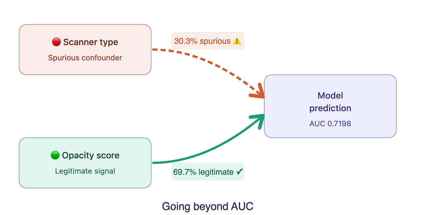
A model can achieve a strong validation performance while learning entirely the wrong things . We demonstrate this by training a ResNet50 on NIH Chest X-ray (14,999 images) to classify an infiltration label reaching an AUC score of 0.7198 — a result most teams would consider a success . Using DoWhy’s Graphical Causal Model, we construct a causal DAG encoding known confounders — scanner acquisition group and image brightness — alongside the legitimate causal path through opacity score. The audit revealed that 30.3% of the modelʼs predictive signal is spurious and if we swapped scanners it shifted mean prediction by +0.12, from 0.4375 to 0.5606, a meaningful difference, because of the properties of a scanner and not pathology. We argue that causal auditing should be a standard practice for any high-stakes ML system, and show that DoWhy makes this accessible.

In 2023, the FDA authorized 221 AI-powered medical devices — up from just six in 2015. Each of these systems makes decisions that affect patients, influencing life or death decisions. But, the question that most teams donʼt ask after getting their accuracy score: “is the model right for the right reasons?”

A model trained on chest X-rays can learn that a particular scanner manufacturer correlates with infiltration diagnoses — not because of pathology or symptoms, but because of the source of the image. It will score well on validation and even pass most audits, but will fail in deployment when it encounters different scanners, and maybe at great cost. This pattern of cross-institutional generalization failure has been documented in medical imaging research [5]. Standard metrics like AUC measure whether predictions correlate with outcomes but say nothing about why. In this article we train a ResNet50 on 14,999 NIH Chest X-ray images to classify infiltration — and then audit it causally using DoWhyʼs Graphical Causal Models. We show that 30.3% of the modelʼs predictive signal is spurious, driven by scanner acquisition artifacts and brightness rather than clinical pathology. More importantly we walk through the exact framework any ML practitioner can use to run audits on their own models.

Background: Spurious Correlations and Causal Inference

Spurious correlations in ML are meaningful relationships that appear in training data but are misleading or non-causal. The model learns these relationships because it tries to reduce error on the training set. In such cases the model may do well in validation or testing, but will fall short of expectations when deployed. This phenomenon — where models exploit unintended statistical regularities — is well documented in deep learning [4] To overcome this, we leverage Judea Pearl’s ladder of causation — three levels of reasoning: seeing (what correlates?), doing (what happens if we intervene?), and imagining (what would have happened differently?). Standard ML metrics operate only at the first level. This article works at all three. It helps us understand relationships between variables using Directed Acyclic Graphs or DAGs. DAGs are visual maps that represent cause and effect relationships between variables.

Image 1 : Causal relationship in weight loss

In the above diagram we try to establish a simple relationship for people who want to lose weight. The more you exercise, the more weight you lose. This is a causal relationship. However, as you go on that journey you find out after initial gains that you canʼt out-train a bad diet. In fact, adjusting your diet alone can help you get better results and even influence your exercise intensity in terms of lean muscle building , replenishment and recovery . In that context diet here becomes our confounding variable — which is a variable that affects both the dependent variable and independent variable. So our Causal graph looks like this now.

Image 2 : Confounder in weight loss

The above DAG now forms the basis to study the relationships in greater detail. It allows us to vary the values of one variable to see the effect on the final outcome. More interestingly it can also evaluate decisions made retrospectively. We use these principles for this study and see that there is a confounding variable — scanner acquisition group, that image appearance and diagnosis rates, creating a spurious path that standard metrics cannot detect. In fact we take the concept of DAG one step further to use GraphicalCausal Models (GCM) from the DoWhy library[3]. It not only maps relationships but also quantifies the strength of each causal path, letting you calculate exactly how much of a model’s prediction flows through spurious vs. legitimate routes. With this framework in place, let’s walk through how we applied it to a real medical imaging classifier.

Training and evaluating an appropriate CNN model

For this study we chose the NIH dataset and used 14,999 chest X-ray images with infiltration label, ~16.6% prevalence (~2,500 positives)[1]. We created 3 splits of 10,499 for training (70%), 2,250 for validation (15%) and the remaining 2,250 (15%)for testing.The labels were derived from NLP analysis of radiology reports rather than manual annotation — a known limitation of this dataset. For a methodological demonstration of causal auditing this is acceptable; any spurious signal we detect reflects real-world label noise practitioners routinely encounter. For model training we use a pre-trained ResNet50 (Residual Network with 50 layers)[2]. It is a Deep convolutional neural network with 50 layers that is widely used for image classification and computer vision tasks. The key innovation for ResNet50 is the use of residual (skip) connections, which allow information to bypass some of the layers, thereby making it easier to train deep networks without the vanishing gradient problem.

Image 3 : Difference between ResNet and a usual CNN

The ResNet50 model that we use is already pre-trained on ImageNet Dataset — million images and about 1000 + object categories. This helps us to use the learned visual features edges, lines, textures, middle layers, learn shapes and object parts etc. on many other image tasks. This saves us immense resources as we donʼt have to train the model from scratch. That done, we now have to train this model on our dataset with a binary-label of “infiltration” : 0/1. As discussed, since we are leveraging a strong pretrained model, we freeze all the layers of the model, except for the last one to be trained according to our dataset and replace the 1000-class fc head with a single neuron for a binary output. Once the training begins we determine that the best AUC value of 0.7198 was reached at epoch 3/10, and thatʼs what we take forward into our study.

Did the model make the decision for the right reasons ?

Now a model with AUC ~0.72 is reasonable. But we ask two questions :

1. How much of that predictive signal comes from the opacity of the lungs x-ray (legitimate) ?
2. How much of that comes from image brightness driven by scanner type (spurious) ?

If the spurious path carries significant influence, we can conclude that the model has learnt the wrong patterns and will fail when deployed at a new hospital with different scanner characteristics.

To determine this we first list and describe the variables that can separate the spurious and the legitimate paths :

1. Infiltration — target, legitimate clinical outcome. It is the presence of fluid, pus, blood, or immune cells — that linger in the lung tissue.
2. Opacity score — legitimate causal path, clinical feature. The presence of the above mentioned substances in lungs changes the density of lungs, becoming more opaque. This opacity is what our ResNet50 looks for and how the model should correctly function.
3. Scanner acquisition group — confounder, spurious path. This node is a representation of the type of scanner that was used when the X-ray was taken on the patient
4. Image brightness — confounder, spurious path. The image brightness, specifically the variability in brightness across images, we believe is caused because of the use of different scanners. Our suspicion is that different scanners produce images of different brightness and this may in-turn impact our modelʼs prediction.
5. CNN model prediction — model output node. Final prediction of our model.

The spurious path is clinically plausible — different hospital systems use different scanner manufacturers, and systematic brightness differences across acquisition groups create a shortcut the model can exploit without ever learning pathology.

We encode this knowledge into the 2 paths for model prediction :

Legitimate : Infiltration → opacity_score→ model_prediction

Spurious : scanner_acquisition_group → image_brightness → model_prediction

Resulting in a causal DAG as follows :

Image 4 : Resulting Directed Acyclic Graph

Applying the Causal Audit

The DAG represents our domain knowledge, and the value of DoWhy actually lies in evaluating the strength of dependencies between the nodes created in the DAG. For this, we wrap the DAG in StructuralCausalModel and let DoWhy’s auto.assign_causal_mechanisms select the right model for each node — empirical distributions for root nodes (no parents), additive noise models for non-root nodes. Once fitted, the GCM moves beyond the qualitative DAG — it can now generate samples that respect the causal structure, simulate interventions, and most importantly, attribute exactly how much of the model’s predictive variance flows through each causal path.

causal_model = gcm.StructuralCausalModel(graph)
gcm.auto.assign_causal_mechanisms(causal_model, data)
gcm.fit(causal_model, data)

The DAG alone tells you which variables are causally related. The fitted GCM tells you how much and what happens when you intervene.

Now we answer the key question : “Of everything that drives model_prediction, how much is causally owned by each variable ?”

Intrinsic Causal Influence answers this by measuring variance in model_prediction attributable to each variable’s ‘noise term’ — i.e the portion that this variable contributes that no other variable can explain.

influence = gcm.intrinsic_causal_influence(
   causal_model,
   target_node='model_prediction',
   num_samples_randomization=200,
)

It’s like if we held everything else fixed and only randomized this variable — how would predictions vary ? Once implemented the following are the results we get.

The Spurious variables image_brightness and scanner_acquisition_group actually account for most of the predictive power while opacity score, the legitimate clinical path, accounts for a smaller share. In fact, when we try to see the total influence of the spurious path using the following code :

spurious = influence['image_brightness'] + influence['scanner_acquisition_group']
total    = sum(influence.values())
print(f'Spurious share: {spurious/total:.1%}')

We see that 30.3% of the influence on model-prediction is dependent on spurious variables.

Infiltration’s near zero score and the higher opacity_score indicates that infiltration’s impact on model_prediction is completely mediated through the opacity_score — as it should be for a legitimate path.

This means the model is partially responding to scanner hardware rather than pathology. A patient scanned on different equipment at a different hospital would receive a meaningfully different prediction, not because their disease changed, but because their scanner did.

The legitimate signal is present but weak relative to the spurious path — which is precisely the problem. The model found a shortcut and leaned on it.

We take this analysis further by introducing the concept of Arrow Strength. It basically quantifies the magnitude of a direct causal effect one variable has on its child using KL divergence and helps answer the key question : If we removed this edge entirely, how much would the distribution of model_prediction change ?

strengths = arrow_strength(causal_model, target_node='model_prediction')

Assessing the Arrow Strengths we output we see that :

The results confirm our concern. The image_brightness → model_prediction edge has an arrow strength of 0.012 — the strongest in the graph — compared to opacity_score → model_prediction at just 0.003, which means that image_brightness will override the influence of opacity_score, a legitimate indicator of infiltration.

Image 5: Arrow Strength graphs

Finally we answer the big question that DoWhy enables us : If we forced every single image to have the brightness of scanner group 1(most common scanner), how would predictions change ?

Intuitively, we would assume that a “good model” would not change in predictions irrespective of which scanner was used, and that is the intention we carry into this analysis. If we do see a significant change or shift in predictions then we can confirm that there is a spurious association.

Specifically we are looking to compare

p(model_prediction) against p(model_predictions | do (brightness = ref)) or observational distribution vs Interventional Distribution.

It is important to state that this is not the same as filtering images by brightness — we are intervening on brightness, cutting the scanner_acquisition_group → image_brightness edge and forcing a fixed value. That distinction is what makes this a causal claim, not a correlational one.

We run the following code block

# Reference: mean brightness of hospital group 1 (largest scanner group)
target_brightness = float(data[data['scanner_acquisition_group'] == 1]['image_brightness'].mean())
print(f'Reference brightness (group 1 mean): {target_brightness:.2f}')
print('Brightness by group (observational):')
print(data.groupby('scanner_acquisition_group')['image_brightness'].mean().round(2))

n_samples = 500

# Draw from observational distribution
obs_samples = gcm.draw_samples(causal_model, num_samples=n_samples)

# Draw from interventional distribution: do(image_brightness = target)
int_samples = gcm.interventional_samples(
   causal_model,
   interventions={'image_brightness': lambda x: np.full(x.shape, target_brightness)},
   num_samples_to_draw=n_samples,
)

print(f'\nObservational mean prediction : {obs_samples["model_prediction"].mean():.4f}')
print(f'Interventional mean prediction : {int_samples["model_prediction"].mean():.4f}')
print(f'Mean shift                     : {int_samples["model_prediction"].mean() - obs_samples["model_prediction"].mean():+.4f}')

And the following output

The difference between observational mean prediction and interventional mean prediction is +0.1132. Under a purely clinical model this should have been 0. The presence or absence of disease should not change just because we swapped a scanner.

Observational vs interventional prediction distribution

Current ML workflows have no standard step that asks why a model makes its predictions before deployment. What we demonstrate here is that this step is both necessary and accessible — a causal DAG, a feature table, and DoWhy’s GCM are sufficient to locate and quantify spurious signals in any supervised model. In cases such as the one demonstrated here, where model failures can cause real life consequences — a causal audit is the difference between deploying a model you understand and one you merely hope will generalize.

The full notebook, including all preprocessing, model training, and causal analysis code, is available as part of the DoWhy open-source library: Notebook: gcm_chest_xray_causal_inference

Conclusion

A model that passes every benchmark can still be wrong for the right reasons — and in high-stakes domains, that distinction is the difference between a tool that helps and one that harms. Hence, it is equally important to run an audit on the model to determine why the predictions were made.

With the knowledge of existing spurious variables we can take steps to nullify their impacts. In this case for example we can retrain the model with randomly varying brightness so that the model does not use it as a shortcut. Even better, we can also look into using causal regularization that penalizes the model during training for using the spurious path in which case running a causal experiment is imperative when we want to move from training/testing to deployment.

When we zoom out of this study, we can see that a model learning un-intended patterns could happen in any applicable domain if we are not careful. Especially, if the data is not curated. You may train a model to rank the best possible resumes for a position, but the model may learn formatting rather than qualifications. In credit card fraud detection, models learn transaction channels rather than behavior. When a model fails in deployment, the cost isn’t just computational — it’s the trust that ML teams have built with clinical partners, business stakeholders, and the people those models affect.

A Causal audit as demonstrated in this study becomes important, not only before deployment of a model but whenever a model is re-trained. To integrate causal audit as part of the ML lifecycle ensures correct decision making, reduces unintended costs and solidifies trust with the external partners. Future work includes extending this audit framework to multi-label classification, testing domain-specific pretrained weights, and integrating causal regularization directly into the training loop.

This analysis is reproducible end-to-end via the contributed DoWhy notebook linked above.

References

[1] Wang, X. et al. (2017). ChestX-ray8: Hospital-scale Chest X-ray Database and Benchmarks. CVPR 2017. https://arxiv.org/abs/1705.02315

[2] He, K. et al. (2016). Deep Residual Learning for Image Recognition. CVPR 2016. https://arxiv.org/abs/1512.03385

[3] Blöbaum, P. et al. (2022). DoWhy-GCM: An Extension of DoWhy for Causal Inference in Graphical Causal Models. arXiv. https://arxiv.org/abs/2206.06821

[4] Geirhos, R. et al. (2020). Shortcut Learning in Deep Neural Networks. Nature Machine Intelligence. https://arxiv.org/abs/2004.07780

[5] Zech, J.R. et al. (2018). Variable generalization performance of a deep learning model to detect pneumonia in chest radiographs: A cross-sectional study. PLOS Medicine. https://doi.org/10.1371/journal.pmed.1002686