🚀 Inside Mistral 7B: Following a Single Token Through the Entire Model (With Real Tensor Shapes!)

🤔 Ever Wondered What Actually Happens Inside an LLM?

When people talk about Large Language Models, you’ll often hear terms like:

• Attention
• Query, Key, Value
• Transformer
• Self-Attention
• KV Cache
• Logits

But what do these things actually look like inside a real model?

Let’s take a real-world model:

Mistral 7B Instruct v0.3

And follow a sequence through the entire model step by step, tracking:

✅ Tensor shapes ✅ Matrix multiplications ✅ Attention calculations ✅ MLP operations ✅ Next-token prediction

By the end, you’ll understand exactly how a prompt becomes a response. 🎉

🏗️ The Architecture We Are Exploring

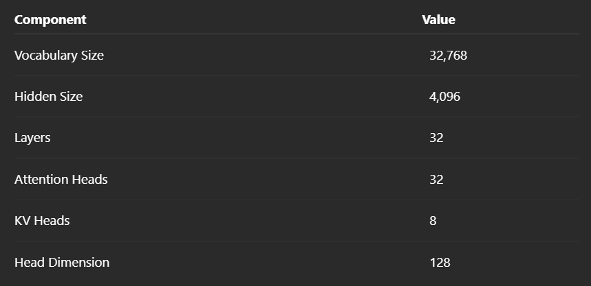
Here’s the important part of Mistral 7B:

Embedding(32768, 4096)

q_proj: 4096 → 4096
k_proj: 4096 → 1024
v_proj: 4096 → 1024
o_proj: 4096 → 4096

gate_proj: 4096 → 14336
up_proj:   4096 → 14336
down_proj: 14336 → 4096

32 Decoder Layers

Important numbers:

🎯 Let’s Use a Real Example

Suppose our prompt contains exactly:

100 tokens

For simplicity:

Batch Size = 1
Sequence Length = 100

Initial shape:

[1, 100]

Meaning:

1 sequence
100 tokens

🤝 Single Token vs 100 Tokens

Throughout this article we’ll compare:

This makes it easier to understand how tensor dimensions grow.

📚 Step 1: Embedding Lookup

The embedding table is:

Embedding(32768, 4096)

Think of it like a giant dictionary:

32768 words
4096 numbers per word

Each token gets converted into a vector.

Single Token

Input:
[1]

Output:
[1, 4096]

100 Tokens

Input:
[1, 100]

Output:
[1, 100, 4096]

Now every token is represented by 4,096 learned numbers.

🎉 Congratulations! The model can finally understand numbers instead of raw token IDs.

🔍 Step 2: Create Queries (Q)

The Query projection is:

q_proj
4096 → 4096

Weight matrix (Wq):

[4096 × 4096]

Single Token

[1 × 4096]
×
[4096 × 4096]
=
[1 × 4096]

100 Tokens

[1 × 100 × 4096]
×
[4096 × 4096]
=
[1 × 100 × 4096]

🔑 Step 3: Create Keys (K)

k_proj
4096 → 1024

Weight matrix (Wk):

[4096 × 1024]

Single Token

[1 × 4096]
↓
[1 × 1024]

100 Tokens

[1 × 100 × 4096]
↓
[1 × 100 × 1024]

📦 Step 4: Create Values (V)

v_proj
4096 → 1024

Weight matrix (Wv):

[4096 × 1024]

Single Token

[1 × 1024]

100 Tokens

[1 × 100 × 1024]

At this point we have:

Q = [1 × 100 × 4096]
K = [1 × 100 × 1024]
V = [1 × 100 × 1024]

🧩 Step 5: Split Into Attention Heads

Mistral uses:

32 Query Heads
8 KV Heads

Head size:

4096 ÷ 32 = 128

Query Heads

[1 × 100 × 4096]
↓
[1 × 32 × 100 × 128]

Key Heads

[1 × 100 × 1024]
↓
[1 × 8 × 100 × 128]

Value Heads

[1 × 8 × 100 × 128]

🤯 Why Only 8 KV Heads?

This is called:

Grouped Query Attention (GQA)

Instead of storing:

32 Query Heads
32 Key Heads
32 Value Heads

Mistral stores:

32 Query Heads
8 Key Heads
8 Value Heads

Result:

✅ Less memory ✅ Faster inference ✅ Smaller KV Cache

Very clever engineering! 🚀

🌀 Step 6: Rotary Positional Embeddings (RoPE)

RoPE injects position information.

Without it:

Token 1
Token 50
Token 100

would all look similar.

RoPE teaches the model:

This token came before that token.

Important:

📏 Tensor shapes do NOT change and this will get applied on Q and K.

🧠 Step 7: Compute Attention Scores

This is where the magic happens.

For one head:

Q = [100 × 128]

K = [100 × 128]

Compute:

Q × Kᵀ

Shape:

[100 × 128]
×
[128 × 100]
=
[100 × 100]

🎯 What Does 100×100 Mean?

Each row:

Current token

Each column:

Token being attended to

Example:

Token 57
asks:
"Which previous tokens are important?"

The answer becomes one row in the attention matrix.

🤯 Attention Matrix Size

One head:

[100 × 100]

32 heads:

[32 × 100 × 100]

Add batch dimension:

[1 × 32 × 100 × 100]

This is the famous attention matrix.

🎲 Step 8: Softmax

Softmax converts raw attention scores into probabilities.

Example:

Before:
[5, 2, 1]
After:
[0.84, 0.11, 0.05]

Shape remains:

[1 × 32 × 100 × 100]

🎨 Step 9: Apply Attention To Values

We now combine attention scores with V.

For one head:

Attention
[100 × 100]
×
Value
[100 × 128]
=
[100 × 128]

Output:

[100 × 128]

for each head.

🔗 Step 10: Concatenate All Heads

32 heads:

32 × 128 = 4096

Combine:

[1 × 32 × 100 × 128]
↓
[1 × 100 × 4096]

Now every token has information gathered from all attention heads.

🎛️ Step 11: The Mysterious o_proj Layer

Many engineers first hear about:

Wq
Wk
Wv

But then suddenly see:

o_proj

and get confused.

What Is o_proj?

Think of attention heads as specialists:

👨‍💻 Head 1 → Code expert

📚 Head 2 → Language expert

🧮 Head 3 → Math expert

🎨 Head 4 → Creativity expert

…

After attention:

[Head1 | Head2 | Head3 | ...]

are simply stacked together.

o_proj mixes all those opinions together.

Weight:

[4096 × 4096]

Input:

[1 × 100 × 4096]

Output:

[1 × 100 × 4096]

Same shape.

Different information.

✨ This is where all attention heads get blended into a unified representation.

➕ Step 12: Residual Connection

Transformer says:

Don’t throw away the original information!

So:

Attention Output
+
Original Input

Result:

[1 × 100 × 4096]

🧠 Step 13: MLP — The Model’s Brain

Attention is communication.

MLP is thinking.

This part is actually larger than attention.

Gate Projection

4096 → 14336

Shape:

[1 × 100 × 14336]

Up Projection

4096 → 14336

Shape:

[1 × 100 × 14336]

SwiGLU

Mistral uses:

SiLU(gate) × up

Shape remains:

[1 × 100 × 14336]

Down Projection

14336 → 4096

Result:

[1 × 100 × 4096]

🔁 Repeat 32 Times

Everything we discussed happens:

32 times

One decoder layer after another.

Shape stays:

[1 × 100 × 4096]

throughout the entire model.

Only the understanding becomes richer.

🏁 Final Layer: LM Head

Weight:

[4096 × 32768]

Input:

[1 × 100 × 4096]

Output:

[1 × 100 × 32768]

🤔 Why 32,768?

Because:

Vocabulary Size = 32,768

The model gives a score for every possible token.

🎲 Example Logits

For the last token:

Paris   → 12.5
London  → 4.2
Berlin  → 1.8
Rome    → 0.5

These are called:

Logits

Not probabilities yet.

🎯 Softmax Converts Logits To Probabilities

Paris   → 82%
London  → 10%
Berlin  → 5%
Rome    → 3%

Now we can choose the next token.

🏆 How Is The Next Token Selected?

The model only looks at:

output[:, -1, :]

which means:

Last token
All vocabulary scores

Shape:

[32768]

Then one of these methods is used:

Greedy

Pick highest probability

Sampling

Randomly sample
based on probability

Top-K

Keep top K tokens

Top-P

Keep tokens whose cumulative probability reaches P

🔄 The Generation Loop

while not finished:
  logits = model(tokens)
      last_logits = logits[:, -1, :]
      probs = softmax(last_logits)
      next_token = sample(probs)
      tokens.append(next_token)

The model keeps repeating this process until:

✅ EOS token appears

or

✅ Maximum length is reached

🎉 Final Takeaway

A Transformer like Mistral is surprisingly elegant:

1️⃣ Convert tokens into vectors

2️⃣ Create Queries, Keys, and Values

3️⃣ Build attention scores

4️⃣ Gather information from other tokens

5️⃣ Mix attention heads with o_proj

6️⃣ Think using the MLP

7️⃣ Repeat 32 times

8️⃣ Produce vocabulary scores

9️⃣ Pick the next token

🔟 Repeat again and again until a full response is generated

And that’s how a simple prompt turns into a detailed answer, one token at a time. 🚀