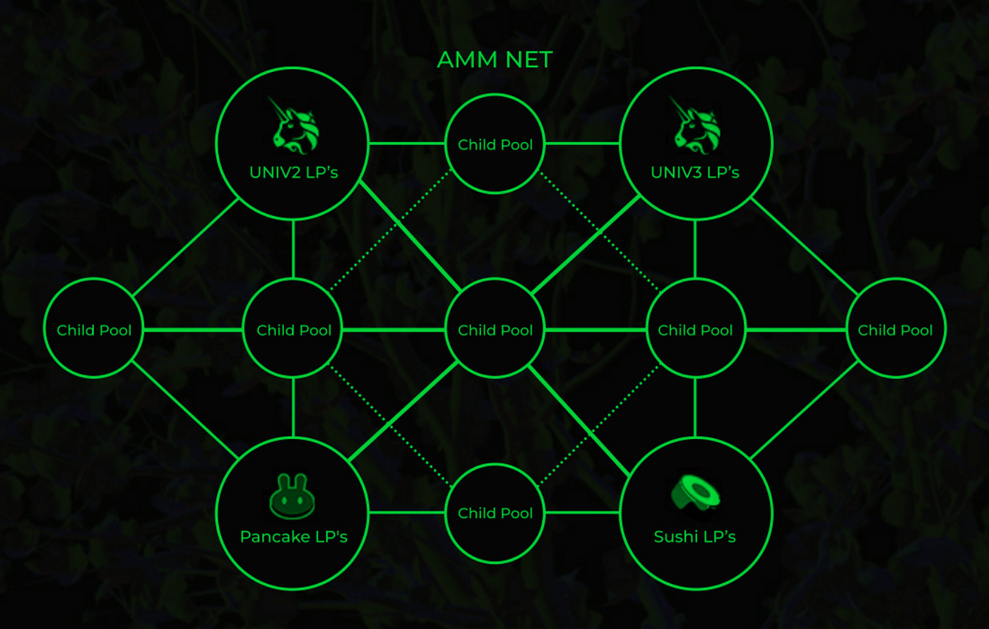
Source: https://pachira.finance

Liquidity Trees: The Next Epoch of DeFi

• Introduction to a new class of DeFi primitives called Liquidity Trees
• Next chapter in the evolution of Automated Market Makers (AMMs)
• Liquidity Trees address a critical market inefficiency thus increasing revenue for liquidity providers

1. Preamble

In this article we will be discussing a new class of DeFi primitives which we have defined as Liquidity Trees. These primitives serve as the core feature behind the soon-to-be released Pachira token supported by SYS Labs.

I have been eagerly waiting about a year to write about this topic since it was first conceptualized (ie, June 2023). Prior to that, myself and cyotee (ie, Liquidity Tree co-inventor and former lead dev from OympusDAO) spent about a year-and-a-half prior doing a much exploratory work (ie, since early 2022). So in all, it’s been nearly 2.5 years of research and development.

In my ETHDenver 2024 talk, which can be considered our first formal public debut of this primitive, I proclaimed that Liquidity Trees will define the next epoch in the evolution of DeFi. I noticed that a couple of others in the community picked this phrase out of the talk and ran with it in various tweets and online discussions. I found this somewhat interesting, because when I perceive this idea, that’s the way I look at it. Hence, as my first introductory article on Liquidity Tree primitives, I thought this would be fun way to pierce into this new and exciting concept. I was cautioned by other members of my team at SYS Labs to keep this article high level, hence this will be the intension as the first step in chronicling this out.

2. Evolution of the Automated Market Maker

The DeFi story really begins with a 2016 Reddit post by Vitalik Buterin (ie, the founder of Ethereum), where he proposed his raw idea of the automated market maker (AMM). A year later, Hayden Adams began working on turning this idea into a functional product and founded Uniswap.

2.1 First Generation AMMs: Constant Product Market Maker

An AMM protocol is the mechanism used by decentralized exchanges (DEXs) and was first introduced by Uniswap, which was launched on the Ethereum mainnet in November 2018. These DEXs consist of liquidity pools (LPs) represented by various trading pairs (eg. ETH/USDC, ETH/WBTC, etc.) acting as the AMM. Trading activity within these LPs are governed via smart contract through the constant product trading (CPT) formula (ie, xy = k).

2.3 First Generation AMMs: Constant Mean Market Maker

In Sept 2019, Balancer Labs published their whitepaper detailing the constant mean market maker, which launched in March 2020. This can be effectively seen as an extension of the constant product market maker idea to include liquidity pools with N assets (ie, (x0x1 … *xN)^(1/N)=k ) with arbitrary weights.

2.4 Second Generation AMMs: Hybrid-CPMM

The first wave of innovations brought issues such as slippage, impermanent loss, and capital efficiency. Hence, with the advent of crypto summer of 2020 began a new generation of AMMs with the introduction of Curve’s Stableswap. This is where they had the insight of combining the constant mean market maker (CMMM) and constant sum market maker (CSMM) into a Hybrid-CPMM. The CSMM has the attribute of producing little slippage during trades, while the CMMM ensures that there is enough depth in the market to facilitate the trade. Hence, Stableswap’s solution is most desirable for trading of stable tokens (eg, USDC, USDT) as provides a highly efficient mechanism to mitigate slippage while ensuring efficient liquidity provision.

2.4 Second Generation AMMs: Virtual Automated Market Maker

Inspired by first generation AMMs like Uniswap coupled with the idea of creating synthetic assets with Synthetix, Perpetual Protocol released the Virtual Automated Market Maker (vAMM) in December 2020. Rather than swapping the actual asset, vAMMs are used to swap virtual assets such as derivative contracts. By utilizing virtual assets, vAMMs provide more capital efficiency and better pricing than first generation AMMs.

2.4 Second Generation AMMs: Lesser known primitives

There are other second generation AMMs worth honorable mention, all addressing issues with impermanent loss and capital efficiency. Bancor introduced automated token trading and Single-Sided Staking. Sushiswap introduced the concept of liquidity mining. Also during this period we have the advent DEX aggregators like 1Inch, Paraswap and OpenOcean.

2.4 Third Generation AMMs: Concentrated Liquidity Market Maker

In May 2021, Uniswap launched V3 as an upgrade to address the lazy liquidity problem, thus introducing the concentrated liquidity market maker (CLMM) protocol. The main idea behind this upgrade was to concentrate the liquidity within the active trading band, which virtually deepens the order book to make more liquidity available for trading; see Fig 1 for more detail. This protocol was arguably the first to address market efficiency through the AMMs liquidity frequency distribution.

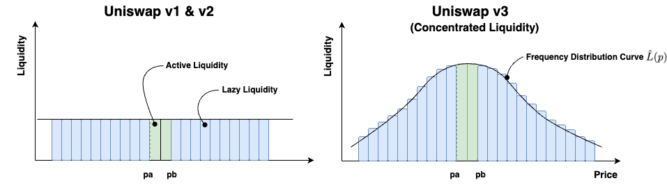
Fig. 1 Comparing liquidity frequency distributions of Uniswap V2 and V3 highlighting advantage of using CLMM

In our ETHDenver talk, we began discussing how the inactive capital within Uniswap V2, known as Lazy Liquidity, which sits outside the active trading range, does not earn yield. This is what’s known as poor capital efficiency. Uniswap V3 addresses this issue by adjusting the liquidity frequency distribution by concentrating liquidity around its active trading region (Pa, Pb) as shown in Fig 1. By doing this, the order book within the liquidity pool (LP) is deepened virtually, thus providing more capital to make larger trades. This is illustrated with the shifting price curve in Fig 2. According to Uniswap, this design enhancement can provide up to 4000x capital efficiency relative to Uniswap V2.

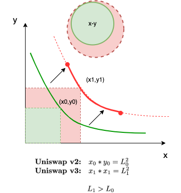
Fig 2. Market depth is increased virtually when going from Uniswap V2 (green) to V3 (red)

3. Networking AMMs using Liquidity Trees

In the previous section we chronicled a brief overview of the evolution of AMM protocols. The unifying characteristic that all the aforementioned have is that they are all single AMM protocols. In this section, we are going to be talking about networks of AMMs, or AMM Nets for short. When enshrined into contract code, AMM Nets open a pandoras box of opportunities, as all the aforementioned protocols mentioned within the last section can be configured into an AMM Net. Liquidity Trees can be considered the simplest class of AMM Nets, and we will be highlighting the advantages of such in this discussion.

If we revisit concentrated liquidity distribution of Fig. 1, the question that we would like to address is how does one employ the capital outside the active trading band so that it is simultaneously earning a return; see Fig 3. We call this inactive region, stagnant liquidity.

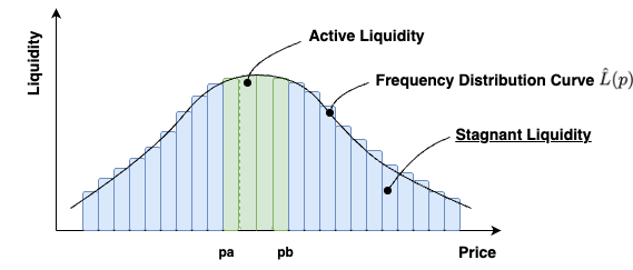
Fig 3. Stagnant liquidity outside the active trading band (Pa, Pb) within CLMM liquidity frequency distribution

If we reference Fig 3, we address the issue of treating the remaining liquidity outside the active trading band as the stagnant liquidity problem. Unlike addressing this issue using a single LP, as referenced throughout the evolution of the AMM, we address the problem using networks of LPs, called Liquidity Trees.

3.1 Let’s include a new dimension (crucial for understanding)

I’ve been told by many degens that grasping this concept can be difficult. However, I implore you to not skim over this crucial step, and take the necessary pause and think about what we are doing here. If you can conceptually grasp this part, and (more importantly) why we are doing it, then extending the solution into more general representations is merely step and repeat. So let’s take the common CPT xy price curve, shown in Fig 2, and extend by including a new dimension as shown in Fig 4.

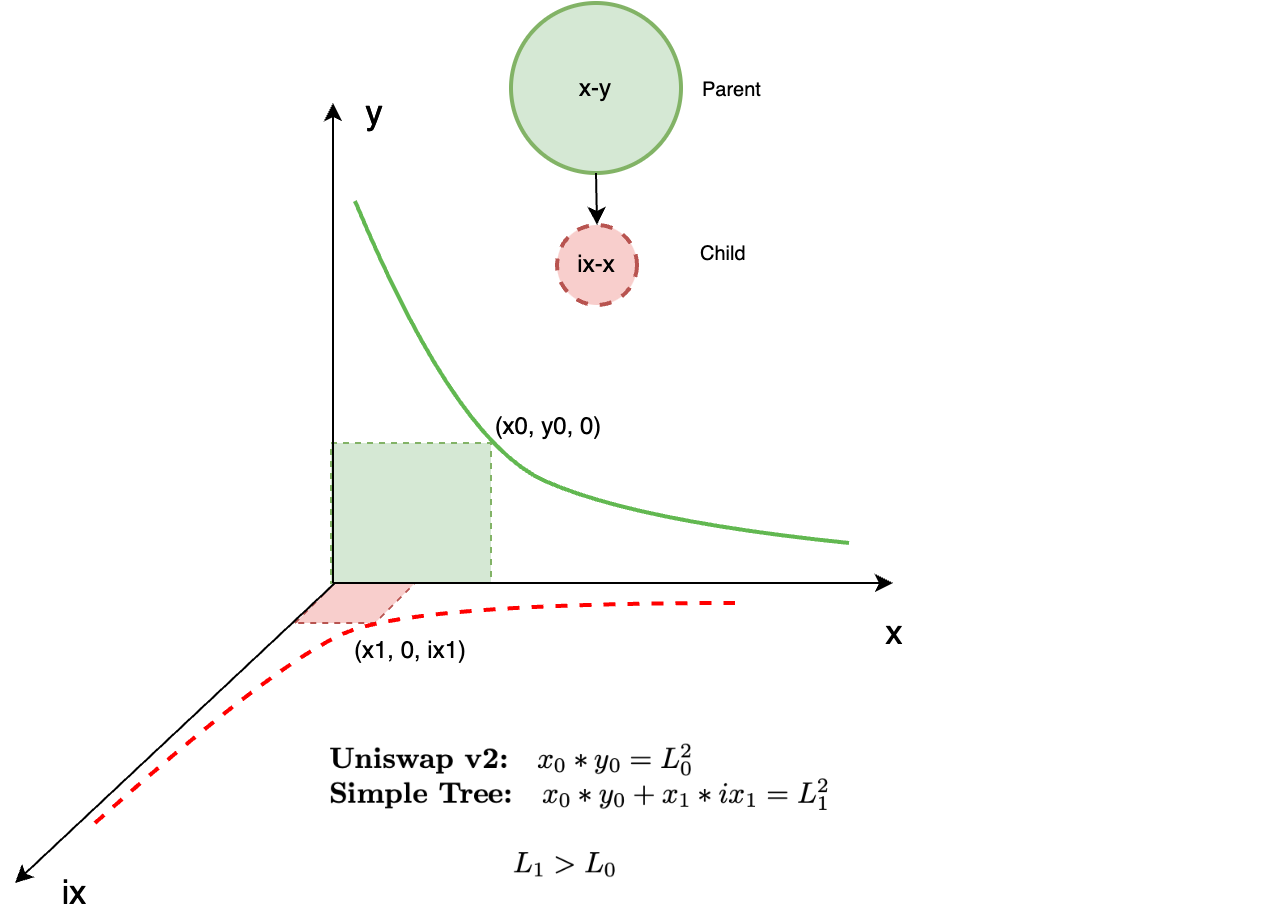
Fig 4. To form a Simple tree, we index x from our original parent LP (green) to create another dimension (ix), and pair back with x to form a new child LP (red)

Instead of thinking in terms of x and y, like we would with the standard CPT formula, we are now thinking in terms of x, y and indexed x, otherwise known as ix. When we say indexing, we use the economic definition, which is compiled economic data into a single metric or measurement. In the case of Liquidity Trees, our economic data is a quantity of LP tokens, measured in terms of either one of the two assets (x or y) as shown in Fig 5. For instance, say we have a USDC/ETH LP and take 10 LP tokens from that pool. We index those 10 LP tokens in terms of USDC or ETH in the form of index tokens defined as iUSDC or iETH. Therefore, as the price of USDC/ETH changes, the quantities of iUSDC or iETH changes as well!

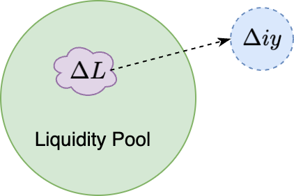
Fig 5. CPT Indexing Problem: given a position ΔL, what is the indexed value in only one of the two pairing assets

Addressing the CPT indexing problem typically involves solving a linear system of equations, and you can read more about that problem in a previous article of mine titled: *The Uniswap Indexing Problem. At the time when we released this article last year, it was pretty much crickets from the community because we hadn’t revealed the gravitas behind it, until now. Without defining and addressing that problem first, we cannot implement a Liquidity Tree.*

So let’s recap; to create a Liquidity Tree, we need to take the two LP assets (eg, x and y) and a quantity of LP tokens from its pool and index them into either ix and/or iy. These index tokens are derived from our LP tokens, which are continually rebased into quantities of x and/or y, which are called continual rebased index tokens (CRITs). These CRITs are placed back on the market to form a child LP, and are paired back with one of the original assets x or y from our parent LP; for example see Fig 4.

Fig 4 depicts the most rudimentary of Liquidity Trees called a Simple Tree, which consists of one parent and one child LP. If we index x as ix and pair with x, we can represent as curves on the x-y plane for the parent LP and on the ix-x plane for the child LP. Likewise, we can also represent as a computational tree, where nodes represent LP operations and arcs between the nodes represent indexed liquidity transiting from the parent to the child LP.

3.2 Why include these new dimensions?

The short answer as to why we include these new dimensions is to earn higher yield from our investment. When we invest into a LP, we receive LP tokens and expect to earn a return from that investment by collecting a share of the trading fees that accrues over time. With a Liquidity Tree, we now have the option of minting index tokens from our invested LP tokens and reinvesting them into the child LP. With this approach, our investment is now making a return both from the parent LP and from the child LP, thus generating higher yield. We are effectively investing into an LP, taking a fully collateralized loan from that investment and reinvesting it. Therefore earning yield from both our original investment and the fully collateralized loan. For the intuition behind this idea, see Fig 6.

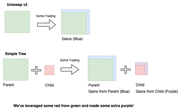
Fig 6. Boxes represent liquidity under CPT curve; creating new market out of index liquidity is a way to address the stagnant liquidity problem; in short, we’ve leveraged some of the green, got red and made some extra purple

Some of you may be wondering, isn’t the DeFi community doing this with DeFi yield farming? In a round about way, yes but technically no. With classic yield farming, LP token positions are handled manually by end users, and must be continually monitored. However, with Liquidity Trees, we have formalized this process and have enshrined it into contract code by employing CRITs, which can only be made possible by first solving the indexing problem. Hence end users do not need to manually manage the positions, which in turn liberates liquidity providers to do more sophisticated things, and also allows designers to build more sophisticated products. As we will show in later articles, with our soon-to-be released Pachira token, this opens a pandoras box of DeFi products that were not made possible before as decentralized institutional technology. Hence, introducing new emergent effects that have the potential to reshape real-world human sociological behavior.

We can see that by using Liquidity Trees, we have addressed the stagnant liquidity problem, as defined in Fig 3. With this process now formalized, we improve market efficiency. So in short, as we outlined in the evolution of the AMM, instead of addressing this problem using single LPs, we address it using networks of LPs called Liquidity Trees. Since we are the first to formalize this class of AMM Nets, we are not just talking about a single new DeFi primitive, but a new class of DeFi primitives which will define the next epoch of DeFi.

3.3 Full Tree

If we expand on the Simple Tree idea discussed in the previous section, Liquidity Trees can be represented as computational graphs where nodes denote LP operations and arcs represent indexed capital transitioning between the parent node and the child. Since there are various types of LPs utilized in DeFi (eg, constant weighted product, composable stable, etc.), for the sake of scope, we will only cover the CPT LP.

For a LP of assets x and y, the maximum combinations of child markets that can be formed are ix-y, ix-x, ix-iy, x-iy, and y-iy. A full Liquidity Tree is when all possible asset combinations are utilized, forming the maximum number of child LPs under the parent; refer to Fig. 7 for a visual representation.

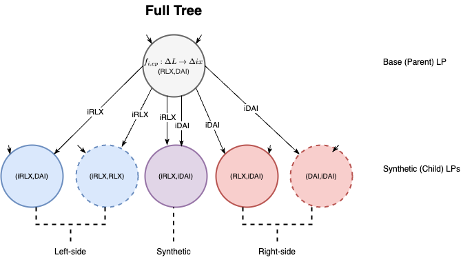
Fig 7. Full CPT liquidity tree represented as a computational tree structure comprised of left-sided, right-sided and synthetic pools

Using other asset combinations, derivations of the full tree from Fig 7 can also be created into various sub-trees; see Fig 8. Simulations have shown us that each of these sub-trees have slightly different nuanced properties which we will discuss in future articles.

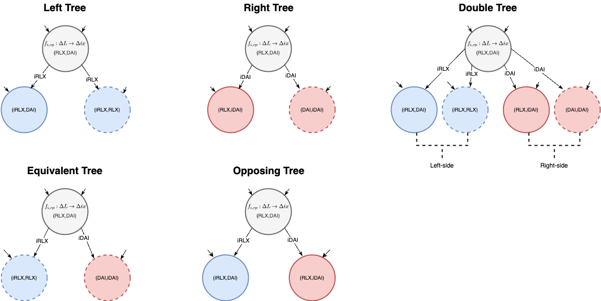
Fig 8. Sub-trees comprised of: (TOP LEFT) left tree; (TOP CENTER) right tree; (TOP RIGHT) double tree; (BOTTOM LEFT) equivalent tree; (BOTTOM CENTER) opposing tree

4. Simulations

In this section we show simulation output using ETH/USDC price data as our input from Jan 2017-Nov 2023. We ran this on a Uniswap V2 Left-tree setup; see Fig 9.

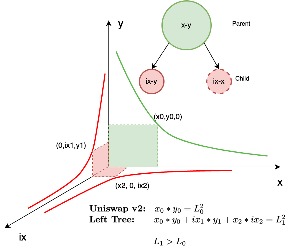
Fig 9. Left tree setup consists of a parent LP (x-y) with its two children (ix-y) and (ix-x)

The swap, deposit and withdraw amounts consist of random non-deterministic samples taken from a Gamma distribution, thus no two simulation runs will produce the same output. To ensure robustness, we ran our simulation through 100 trials and took the medians of the outcomes as displayed in Table 1.

It is important to note that there is an upper bound to the number of minted index tokens that can be deployed into the Liquidity Tree child markets. For instance, if the market cap of our parent pool is $1M USD, then we have access to a maximum of $1M USD that can be minted for index tokens. However in reality, it is highly improbable that a tree’s parent LP will have 100% of its capital deployed into index tokens, as once capital is minted, then it is no longer available for trading. At this stage, we are presuming that it a parent LP will have 10–70% of its capital deployed into index tokens. Which is why we have depicted the red planes of the child LPs in Fig 9 to be considerably smaller than the green plane of the parent LP. Therefore, when we ran these simulations, we conservatively assumed that only 25% of the capital in the parent LP was deployed into the child LPs, as indicated in the first row of Table 1.

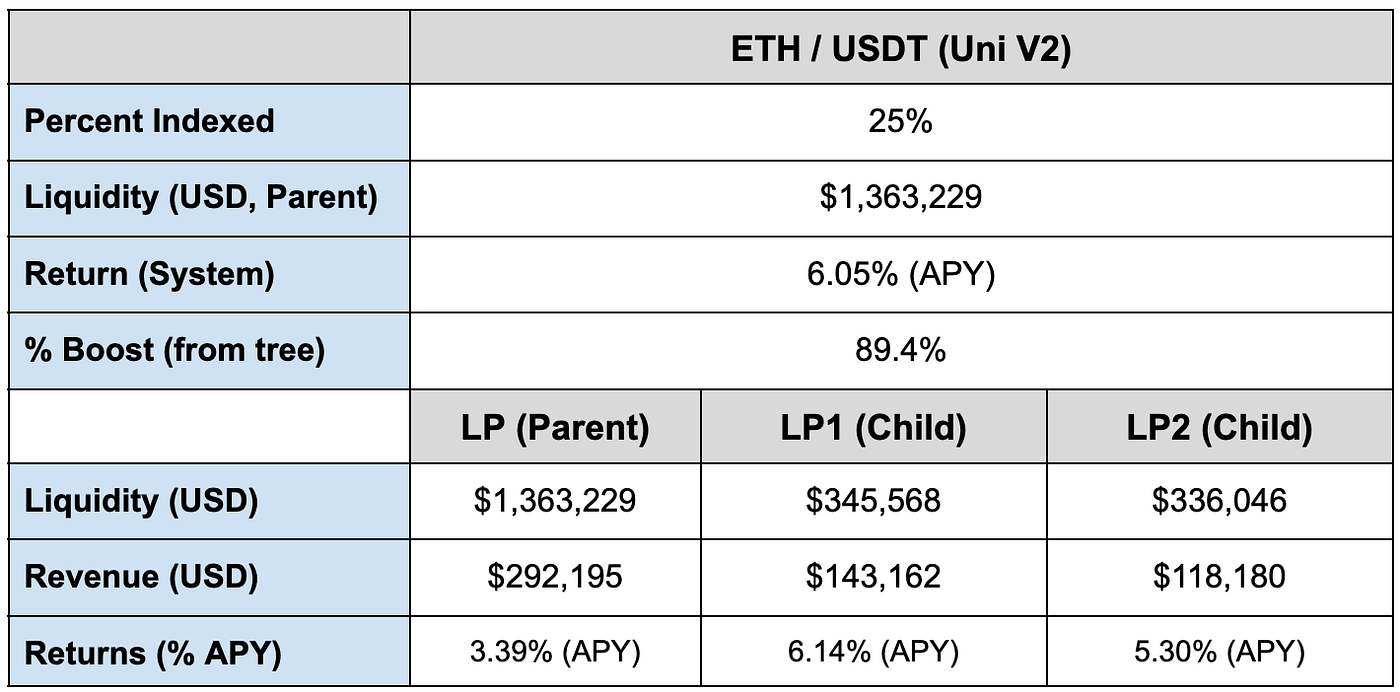
Table 1: Output measured from (N = 100) Left-tree simulation trials using ETH / USD (Jan 2018 to Nov 2023)

An interesting feature worthy of discussion is that APY within the children is always found to be consistently higher than APY of the parent. We found this to be the case, no matter how many times we ran the simulation, what price samples were used, trade volume, or tree configuration employed. This has to do with how the price of index tokens in the child LPs respond to the price of the native tokens within the parent LP. This is because the volatility of the asset prices in the child LPs is more exacerbated than the volatility of the asset prices in the parent LP. Thus higher volatility in the child assets prices presents arbitrage opportunities that get filled by opportunistic agents (eg. trading bots).

Another interesting feature worth noting is because we see higher volatility in child LP asset prices, it is not necessary to mint a large portion of the capital as index tokens to realize a significant performance boost. This is supported by the simulation outcomes presented in Table 1. Here we see that with only 25% of parent capital deployed as index tokens, an 89.4% performance boost is received from the children. More specifically, our results show we receive a 3.39% annual percentage yield (APY) from the parent, and a system-wide 6.05% APY from the tree as a whole.

5. Summary: The Next Epoch of DeFi

We began this article with a preamble followed by a summary of the evolution of the AMM. We concluded that up to this point, the unifying characteristic that all these AMMs have is that they are all single LP protocols. Next, we explore the idea of the AMM Net which is a network of AMMs enshrined into contract code. Within this new class of DeFi primitives, Liquidity Trees can be considered the simplest of such.

We define the stagnant liquidity problem, and show how Liquidity Trees addresses this issue as evidenced through simulation. Liquidity Trees are a good approach to improve market efficiency, thus earning a higher return on capital investment, as shown in Table 1. Liquidity Trees liberate liquidity providers and designers to deploy more sophisticated DeFi strategies and protocols, which we will be discussing with the soon-to-be released Pachira token in the upcoming months. With this, we believe this will also invoke emergent sociological behavior at the institutional level, which will be the subject of much research within SYS Labs in the years to come.

Once the indexing problem is solved for a given AMM, it can be deployed into a Liquidity Tree. Currently, we have solved the indexing problems for the Mooniswap, Uniswap V2 and V3 protocols. So far, we have only discussed this openly with Uniswap V2 and will be delving deeper into this in the upcoming future. We plan on releasing the python code to the Liquidity Tree simulator within the coming months. In the meantime, readers can also checkout DeFiPy which the suite of python tools that our simulator depends on.

In summary, we have presented a new class of DeFi primitives called Liquidity Trees which will define the next epoch of DeFi. This is a high-level introductory article, and we plan on discussing more in-depth technical elements of this topic in future articles to come. If you want to stay up-to-date with this exciting project, you can visit the Pachira project website, or follow me on Twitter/X!

TextBook

If you enjoy my DeFi analytics content, you’ll love the official textbook:

📘 DeFiPy: Python SDK for On-Chain Analytics AMM math • Uniswap V2/V3 • Balancer • Stableswap • liquidity modeling • agents 👉 https://www.amazon.com/dp/B0G3RV5QRB

Visit us at *DataDrivenInvestor.com*

Subscribe to DDIntel *here*.

Join our creator ecosystem *here*.

DDI Official Telegram Channel: https://t.me/+tafUp6ecEys4YjQ1

Follow us on *LinkedIn, [Twitter](https://twitter.com/@DDInvestorHQ), [YouTube](https://www.youtube.com/c/datadriveninvestor), and [Facebook](https://www.facebook.com/datadriveninvestor)*.