Linear Regression Explained: From Theory to Real-World Implementation

Understanding the math, assumptions, and practical steps to predict continuous outcomes with confidence

Predicting the values of dependent continues random variable Y from independent continues random variable X, with the help of a regression function r(x) which takes a value from X and returns a prediction ŷ. Our goal is to find a function r(x) that, for any given x, predicts y as accurate as possible ( ŷ ≈ y ). In statistics, the function that gives the minimum possible bias is :

This is the conditional expectation — the average value of Y when X is fixed at x. It doesn’t mean we predict every single Y exactly(due to noise and randomness it’s hard) but it means we predict the average outcome given X, which is the best we can do without extra information. A simple example,

Yes, there is difference in our prediction values with actual values. In cases where ŷ should be 5,7,9,11,13,15 we gave a prediction 1 unit above or below the value which gave us the Residual Sum of Squares

of 6.0 which is the sum of units our error predictions deviates from true values. So, our statistical function E[Y | X] which says, if there are multiple y values for a single fixed x the best prediction we can make with less error is predicting the average of those y values, which make sense. So, now we are confident that E[Y | X] gives us optimal prediction of random variable Y.

We don’t know what the real shape of E[Y | X] looks like. In theory, it can take any shape with population data:

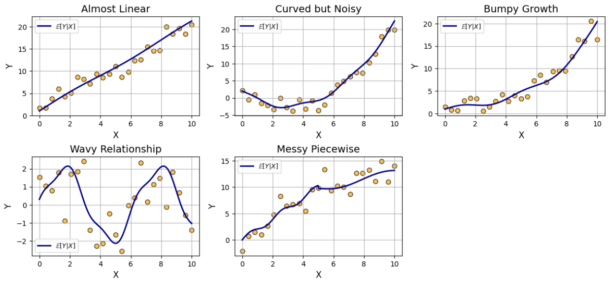
In practice, we only get finite and noisy data points. So we need to approximate E[Y | X] curve.

If you ever used LinearRegression() from scikit-learn package:

from sklearn.linear_model import LinearRegression

model = LinearRegression()
model.fit()
model.predict()

You were agreed with these assumptions:

1. Linearity — Relationship between predictors and response is linear.
2. Independence — Errors are independent from each other.
3. Normality of errors — Errors are normally distributed (mainly for inference).
4. Homoskedasticity — Constant variance of errors.
5. No multicollinearity — Predictors aren’t highly correlated with each other.

Let’s start from scratch and see how this assumptions are helping linear regression to make better predictions and inference.

Linearity because, we assume the variables X and Y have linear relationship i.e. We assume the E[Y | X] is a straight line. The straight line formula,

• β1 is slope
• β0 is intercept

Just like any other parametric model where we assume our data follows some distribution (like normal, binomial, etc) and make predictions on the distribution, here we assume our E[Y | X] follows a straight line and make prediction using that straight line. This is the reason for calling linear regression a parametric model.

The parametric idea is also same, just like we estimate mean and variance in normal distribution, we can estimate our β0 and β1 values:

we can use either MLE or Ordinary Least Square(OLS) method to find our point estimates.

In OLS :

set the above formula to 0 w.r.t β0 and β1:

solving this will result in:

In MLE:

we can say,

Assume error forms a normal distribution with mean 0 and an unbiased error variance:

Therefore:

The likelihood function would be:

The log likelihood would be:

The log likelihood increases if the term:

Decreases. This term is the RSS, the thing we shrink in Least Squares. Under the normality assumption, boosting the log-likelihood just means cutting down this RSS — a neat case where MLE and Least Squares end up doing the same thing. So, taking the derivative of log likelihood w.r.t β0 and β1 would give us the same formulas.

Let’s apply this estimated β0 and β1 to our E[Y | X] example and see if the RSS is 6.0 as it will be if the least square parameters (β0, β1) finds out the best fitting line that gives minimum error:

import numpy as np

x = np.array([1, 1, 1, 2, 2, 2, 3, 3, 3])
y = np.array([5, 6, 7, 9, 10, 11, 13, 14, 15])

# Least Squares Estimates
beta1 = np.sum((x - np.mean(x)) * (y - np.mean(y))) / np.sum((x - np.mean(x))**2)
beta0 = np.mean(y) - beta1 * np.mean(x)

# Fitting A Line
y_pred = beta0 + beta1 * x

RSS = np.sum((y - y_pred)**2)

print('Statistical optimal predictions: [6., 6., 6., 10., 10., 10., 14., 14., 14.]')
print('Model Prediction:', y_pred)
print('RSS: ', RSS)

Statistical optimal predictions: [6., 6., 6., 10., 10., 10., 14., 14., 14.]
Model Prediction: [ 6.  6.  6. 10. 10. 10. 14. 14. 14.]
RSS:  6.0

import matplotlib.pyplot as plt

plt.scatter(x, y, color='royalblue', edgecolor='black', s=50, alpha=0.8, label='Data Points')
plt.plot(x, y_pred, color='darkred', linewidth=2.5, label='Fitted Line')

plt.xlabel("X", fontsize=12)
plt.ylabel("Y", fontsize=12)
plt.title("Linear Regression Fit", fontsize=14)
plt.legend()
plt.grid(True, linestyle='-.', alpha=0.6)
plt.tight_layout()
plt.show()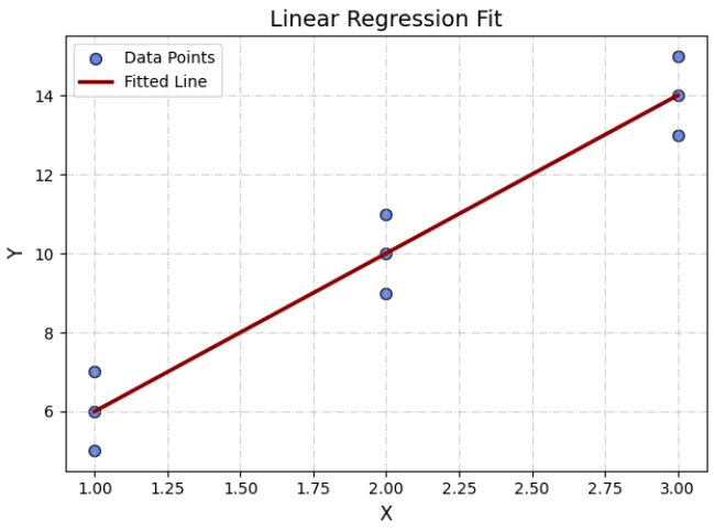

residuals = y - y_pred
plt.figure(figsize=(7, 5))
plt.scatter(y_pred, residuals, alpha=0.9, s=50, edgecolor='black', color='royalblue')
plt.axhline(0, color='darkred', linestyle='--', linewidth=1.5, label='Zero Residual Line')

plt.xlabel("Predicted Values", fontsize=12)
plt.ylabel("Residuals", fontsize=12)
plt.title("Residuals vs Predicted Values", fontsize=14)
plt.grid(True, linestyle='-.', linewidth=0.5, alpha=0.7)
plt.xticks(fontsize=10)
plt.yticks(fontsize=10)
plt.legend()
plt.tight_layout()
plt.show()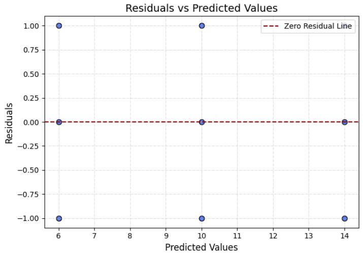

The way the least square estimates predictions is exactly similar to E[Y | X] is because least square parameters are designed in a way to reduce the squared error (RSS) , statistically the way to reduce the error when you have multiple y’s for a single x is predicting the mean of those values.

I like using R square score to judge the regression model performance, you can skip the following explanation if you already know how R square works

R square :

We know that,

And Total Sum of Squares(TSS) be the total variability in the dependent variable y. If we have a base model that always predicts mean of y for every data point x, then TSS can also be described as “The total variability explained by that base model compared to having no model at all”.

If we perform,

Since, RSS is the variability our model didn’t explained.

• The resulted scalar will be 1 if our model performed same as base model (RSS = 1, TSS = 1) this means every ŷ our model predicted, is the mean of the dependent variable ȳ (ŷ = ȳ), which also means our model didn’t learned (or) didn’t found any patterns from X to understand variability in Y and just returning the mean of Y.
• Scalar can be greater than 1 if model performs even worse than predicting just ȳ.
• Scalar goes near 0 when numerator RSS goes down, means model explaining most of the variability in Y.

We can invert the scale by,

Now,

• R square < 0 performing worse than base model
• R square = 0, our model isn’t explaining any variability in Y values compared to base model
• R square = 0.5, our model is explaining 50% more variability compared to base model
• R square = 1, our model is explaining all the variability in Y. This is not common, especially in regression models where there is noise

Finding R square of our straight line:

RSS = np.sum((y - y_pred)**2)
TSS = np.sum((y - np.mean(y))**2)

R_square = 1 - (RSS/TSS)

print(f"R square : {R_square:.4f}")

R square : 0.9412

This means the model is explaining around 94% of the variability in Y compared to base model which predicts 10 all-the-time in our case.

Linear regression does give good prediction score but using “accuracy” as the metric for linear regression doesn’t really make sense — it’s a parametric model, built more for inference and interpretability than for raw prediction scores.

We can perform techniques like finding Confidence Intervals for parameters and predictions, Hypothesis testing, Interpreting our parametric results, p-values. For our example data, to see the 95% confidence interval for our slope, we can use a direct formula for variance of β1 without performing any bootstrap:

var = (1/(len(y) - 2)) * np.sum((y - y_pred)**2) # error variance

var_beta1 = var/np.sum((x - np.mean(x))**2)

se_beta1 = var_beta1 ** 0.5

alpha = 1 - 0.95

beta1_interval = [beta1 - norm.ppf(1 - alpha/2) * se_beta1, beta1 + norm.ppf(1 - alpha/2) * se_beta1]

print(f"Standard Error of β1 : {se_beta1:.2f}")
print(f"Estimated slope : {beta1}")
print(f"With 95% confidence this interval contains the true slope : [{beta1_interval[0]:.2f}, {beta1_interval[1]:.2f}]")

Standard Error of β1 : 0.38
Estimated slope : 4.0
With 95% confidence this interval contains the true slope : [3.26, 4.74]

From *Confidence Is The New Truth we saw that for the normal interval to work, the sampling distribution needs to be approximately normal. That means the sampling distribution of our slope should be normal — which it is, since we assumed Normality of Error. And because β1*​ is just a linear combination of those errors, that normality carries over directly to the slope. In other words, if the errors are normal, our slope is normal too — making the whole confidence interval story click.

We’ve got the slope and intercept, we can now make predictions on new data. That’s one big reason we don’t stop at just writing E[Y∣X] for our sample — we actually fit a model so it can work beyond the data we’ve already seen.

x_new = 5

y_pred_new = beta0 + beta1 * x_new

print(f"For x:{x_new} y is {y_pred_new}")

For x:5 y is 22.0

The example we took is very convenient for our least squares estimates to predict near true values since the growth or slope of the means is constant 4. This is easy for a straight line to handle. What if i nudge the values a bit, breaking the constant slope? Like

x=np.array([1,1,1,2,2,2,3,3,3])
y=np.array([5,6,7,9,10,11,17,18,19])

Fitting a straight line through 6, 10, 18 is not possible with just 3 units distance in x-axis. The RSS increases, The Error Variance Increases, The Standard Error Increases, The Uncertainty Increases, The width of CI increases. Let’s see if it happens:

x=np.array([1,1,1,2,2,2,3,3,3])
y=np.array([5,6,7,9,10,11,17,18,19])

beta1_m2 = np.sum((x - np.mean(x))*(y - np.mean(y))) / np.sum((x - np.mean(x))**2)
beta0_m2 = np.mean(y) - beta1_m2 * np.mean(x)

y_pred = beta0_m2 + beta1_m2 * x

RSS = np.sum((y - y_pred)**2)

print('Model Prediction:', y_pred)
print(f"RSS : {RSS:.2f}")
print(f'Slope: {beta1_m2}')

Model Prediction: [ 5.33333333  5.33333333  5.33333333 11.33333333 11.33333333 11.33333333 17.33333333 17.33333333 17.33333333]
RSS : 14.00
Slope: 6.0

plt.scatter(x, y, color='royalblue', edgecolor='black', s=50, alpha=0.8, label='Data Points')
plt.plot(x, y_pred, color='darkred', linewidth=2.5, label='Fitted Line')
plt.xlabel("X", fontsize=12)
plt.ylabel("Y", fontsize=12)
plt.title("Linear Regression Fit", fontsize=14)
plt.legend()
plt.grid(True, linestyle='-.', alpha=0.6)
plt.tight_layout()
plt.show()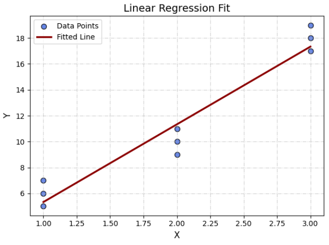

The RSS is increased and we can see the line tried to fit the updated data points with getting as minimum error as possible.

residuals = y - y_pred
plt.figure(figsize=(7, 5))
plt.scatter(y_pred, residuals, alpha=0.9, s=50, edgecolor='black', color='royalblue')
plt.axhline(0, color='darkred', linestyle='--', linewidth=1.5, label='Zero Residual Line')

plt.xlabel("Predicted Values", fontsize=12)
plt.ylabel("Residuals", fontsize=12)
plt.title("Residuals vs Predicted Values", fontsize=14)
plt.grid(True, linestyle='-.', linewidth=0.5, alpha=0.7)
plt.xticks(fontsize=10)
plt.yticks(fontsize=10)
plt.legend()
plt.tight_layout()
plt.show()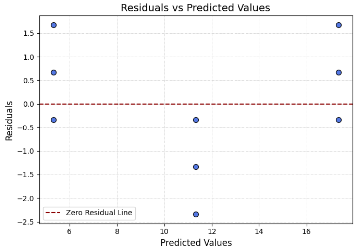

The straight line is not doing a bad job, it’s doing great with its possible physical traits as we can see in the above plot, none of the predicted values have 0 error but it’s the minimum error it could get, satisfying all the data points.

RSS = np.sum((y - y_pred)**2)
TSS = np.sum((y - np.mean(y))**2)

R_square = 1 - (RSS/TSS)

print(f"R square : {R_square:.4f}")

R square : 0.9391

The R square dropped only a little even though the RSS is higher than before, because it is still explaining a lot of variability in the Y values compared to just predicting ȳ.

var = (1/(len(y) - 2)) * np.sum((y - y_pred)**2)

var_beta1_m2 = var/np.sum((x - np.mean(x))**2)

se_beta1_m2 = var_beta1_m2 ** 0.5

alpha = 1 - 0.95

beta1_interval = [beta1_m2 - norm.ppf(1 - alpha/2) * se_beta1_m2, beta1_m2 + norm.ppf(1 - alpha/2) * se_beta1_m2]

print(f"Standard Error of β1 : {se_beta1_m2:.2f}")
print(f"Estimated slope : {beta1_m2}")
print(f"With 95% confidence this interval contains the true slope : [{beta1_interval[0]:.2f}, {beta1_interval[1]:.2f}]")

Standard Error of β1 : 0.58
Estimated slope : 6.0
With 95% confidence this interval contains the true slope : [4.87, 7.13]

Model B has extra residuals compared to model A, and if those residuals increase the spread of errors, they raise the variance. Higher variance means a higher standard Error (as it did for 0.58), which indicates that model B’s β estimates leave more unexplained variation than model A. Higher SE can also increases the width of CI with same confidence.

Take aways until now:

• In linear regression, we assume normality of errors so that the slope’s sampling distribution is normal, enabling valid normal-based confidence intervals.
• The fitted slope and intercept let us predict on new data, unlike simply stating E[Y∣X] for our sample.
• The residual sum of squares (RSS) is what we minimize in least squares — and under normal errors, this is equivalent to maximizing the likelihood.
• Extra residuals can increase the spread of errors, raising variance and standard deviation, which means the model’s β estimates are leaving more variation unexplained.

Let’s see how a straight line is performing compared to E[Y|X] on real world data:

#  LINEAR REGRESSION

import pandas as pd

df = pd.read_csv('weight-height.csv', usecols=['Height', 'Weight'])

train_samples = int(len(df) * 0.7)

samples_idx = np.random.choice(len(df), size=train_samples, replace=False)

df_train = df.iloc[samples_idx]
df_test = df.drop(df.index[samples_idx])

X_train = df_train['Height'].to_numpy()
Y_train = df_train['Weight'].to_numpy()

X_test = df_test['Height'].to_numpy()
Y_test = df_test['Weight'].to_numpy()

X_mean = np.mean(X_train)
Y_mean = np.mean(Y_train)

beta1 = np.sum((X_train - X_mean) * (Y_train - Y_mean)) / np.sum((X_train - X_mean)**2)
beta0 = Y_mean - beta1 * X_mean

Y_pred = beta0 + beta1 * X_train

# Model with E[Y|X] near performance
from scipy.stats import binned_statistic

# Bin the heights and compute average weight in each bin -> E[Y|X]
bin_means, bin_edges, _ = binned_statistic(X_train, Y_train, statistic='mean', bins=50)
# Get the centers of the bin for plotting accuracy
bin_centers = (bin_edges[:-1] + bin_edges[1:]) / 2

Binned statistics group nearby x values into bins, since in regression data we rarely get identical x values repeating. This is about as close as we can get to replicating E[Y|X].

plt.figure(figsize=(8, 5))
plt.scatter(X_train, Y_train, alpha=0.1, label='Training Data')
plt.plot(bin_centers, bin_means, color='black', linewidth=2, label='Estimated E[Y|X] (bin average)')
plt.plot(np.sort(X_train), np.sort(Y_pred), color='red', alpha=0.7,linewidth=2, label='Linear Regression')
plt.xlabel('Height')
plt.ylabel('Weight')
plt.legend()
plt.grid(True)
plt.title('Estimated E[Y|X] vs Linear Regression')
plt.show()

The linear regression model (red line) closely follows the binned estimate of E[Y|X](black line) across the full range of heights, indicating that the linearity assumption holds strongly for this dataset. The small deviations of the binned curve from the straight line are minor and mostly due to local fluctuations in the data rather than systematic bias. The tight clustering of points around both lines suggests low variance and high predictive accuracy, with no visible pattern in residual spread. The model captures the underlying relationship between height and weight very effectively.

RSS = np.sum((Y_train - Y_pred)**2)
TSS = np.sum((Y_train - Y_mean)**2)

R_square = 1 - (RSS/TSS)

print(f"R square : {R_square:.4f}")

R square : 0.8562

The linear regression model capturing around 85% of the variability in the data compared to base model, that’s not bad at all. Let’s see if our assumption of normality in error holds for this data:

import seaborn as sns

residuals = Y_train - Y_pred

plt.figure(figsize=(8, 5))
sns.histplot(residuals, bins=35, kde=True, color="skyblue", edgecolor="black", alpha=0.7)

plt.title("Residuals Distribution", fontsize=16, fontweight='bold')
plt.xlabel("Residual", fontsize=14)
plt.ylabel("Frequency", fontsize=14)
plt.axvline(0, color='red', linestyle='--', linewidth=1.5, label="Zero Residual Line")
plt.legend()
plt.grid()

plt.show()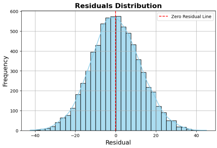

The residuals appear approximately normally distributed, which supports our normality of errors assumption. This means we can confidently apply statistical inference — such as confidence intervals and hypothesis tests — on our model parameters. While normality of errors ensures our parameter estimates follow the distributions we rely on for inference, there’s another equally important assumption: homoskedasticity.

Homoskedasticity:

Homoskedasticity means the variance of the errors should be constant across all values of X. If the spread of residuals changes with X (a “fan” or “cone” shape in a residual plot), we have heteroskedasticity, which can lead to unreliable standard errors and misleading confidence intervals — even if the errors are normally distributed. Which also means error variance (σ²) is only valid for inference(we used error variance in past to get variance of β1) if and only if the variance of the errors at each data point x is constant. Below plots show the text book definition of homoskedasticity and heteroskedasticity.

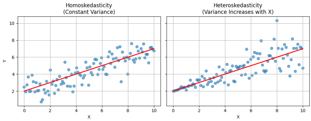
For example, take two x values from the heteroskedasticity plot: x1 = 2 and x2 = 8. After prediction, suppose we get ŷ1 = 3 and ŷ2 = 6, while the actual values are y1 = 2.5 and y2 = 4.

If we construct confidence intervals for these predictions using the error variance from heteroskedastic data, the results may be misleading. Because the variance of errors changes with x, the CI for ŷ1 might be unnecessarily wide (overestimating uncertainty), while the CI for ŷ​2​ might be too narrow (underestimating uncertainty).

In contrast, with homoskedasticity, the error variance is constant and stable across all x values, so doing inference is more reliable. This is the reason why we assume homoskedasticity in linear regression

Note: there are statistical techniques to address heteroskedasticity, but some real world data — such as housing prices, where higher-priced homes have more variability — naturally exhibit it.

We can visualize doing a plot of either ( X vs Residuals) or (Y predictions vs residuals) since ŷ looks similar to x and in multiple regression(regression with more than 1 variable) ŷ can be our go to.

plt.figure(figsize=(8, 5))
sns.scatterplot(Y_pred, residuals, alpha=0.6, edgecolor=None)
plt.axhline(0, color='red', linestyle='--', linewidth=1.5)
plt.xlabel("Predicted Values", fontsize=12)
plt.ylabel("Residuals", fontsize=12)
plt.title("Residuals vs Predicted Values", fontsize=14, fontweight='bold')
plt.tight_layout()
plt.show()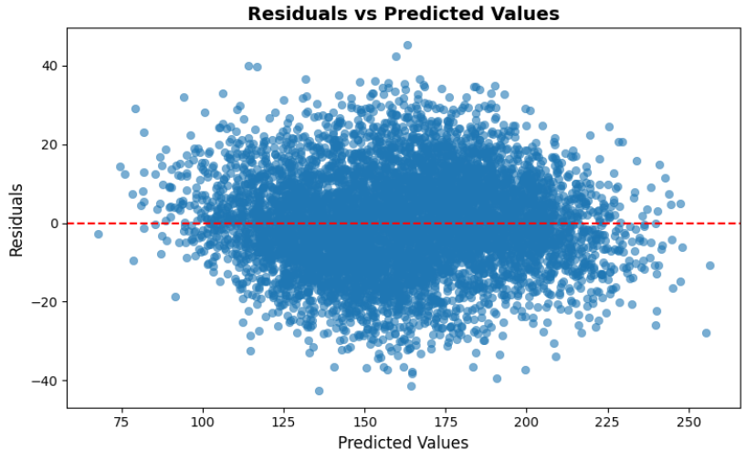

I don’t see any patterns or errors expanding with predicted values all the errors are scattered around the 0 errored line, so we don’t have heteroskedastic data.

VAR = (1/(len(Y_train) - 2)) * np.sum((Y_train - Y_pred)**2)

VAR_BETA1 = VAR / np.sum((X_train - X_mean)**2)

SE_BETA1 = VAR_BETA1 ** 0.5

print(f'A valid variance due to homoskedasticity : {VAR:.4f}')
print(f"Standard Error of parameter β1: {SE_BETA1 :.4f}")

A valid variance due to homoskedasticity : 148.0742
Standard Error of parameter β1: 0.0376

Finding the true β1 (true slope) on true height and weights data would look like:

alpha = 1 - 0.95

beta1_interval = beta1 - norm.ppf(1 - alpha/2)* SE_BETA1, beta1 + norm.ppf(1 - alpha/2) * SE_BETA1

print(f"Our Estimate of true slope : {beta1:.2f}")
print(f"With 95% confidence this interval contains the true slope : [{beta1_interval[0]:.2f}, {beta1_interval[1]:.2f}]")

Our Estimate of true slope : 7.71
With 95% confidence this interval contains the true slope : [7.63, 7.78]

Now we got slope and intercept we can predict weight given height:

X_new = 73.5
Y_new = beta0 + beta1 * X_new

SE_Y_new = np.sqrt(
    VAR * (1 + 1/len(X_train) + (X_new - X_mean)**2 / np.sum((X_train - X_mean)**2))
)

alpha = 1 - 0.95
z = norm.ppf(1 - alpha/2)

ci_lower = Y_new - z * SE_Y_new
ci_upper = Y_new + z * SE_Y_new

print(f'For height of {X_new} the predicted weight is: {Y_new:.2f}')
print(f"95% CI for prediction at X={X_new}: [{ci_lower:.2f}, {ci_upper:.2f}]")

For height of 73.5 the predicted weight is: 216.42
95% CI for prediction at X=73.5: [192.56, 240.28]

The standard error of a new prediction shows how uncertain that prediction is. It combines the natural spread of data points around the regression line, the fact that we estimated the model from limited data, and how far the new input is from the average of what the model has seen before. Predictions for values far from the average come with more uncertainty. We use this standard error to build confidence or prediction intervals — ranges where the actual value is likely to fall.

Now let’s compare our parameters and R square score with LinearRegression() in scikit-learn library.

from sklearn.linear_model import LinearRegression

model = LinearRegression()
model.fit(X_train.reshape(-1, 1), Y_train)

print(f"β1 (sklearn): {model.coef_[0]:.4f}")
print(f"β0 (sklearn): {model.intercept_:.4f}")

print(f"β1 (manual): {beta1:.4f}")
print(f"β0 (manual): {beta0:.4f}")

Y_test_pred = model.predict(X_test.reshape(-1, 1))

rss = np.sum((Y_test - Y_test_pred) ** 2)
tss = np.sum((Y_test - np.mean(Y_test)) ** 2)

model_r2_score = 1 - (rss / tss)

print(f"Model's R square score (sklearn): {model_r2_score:.4f}")

Y_test_pred = beta0 + beta1 * X_test

RSS_test = np.sum((Y_test - Y_test_pred) ** 2)
TSS_test = np.sum((Y_test - np.mean(Y_test)) ** 2)

R_square_test = 1 - (RSS_test / TSS_test)

print(f"Our R square score (manual): {R_square_test:.4f}")

β1 (sklearn): 7.7125
β0 (sklearn): -350.4167
β1 (manual): 7.7125
β0 (manual): -350.4167
Model's R square score (sklearn): 0.8611
Our R square score (manual): 0.8625

Both sklearn’s LinearRegression and our manual calculation gave almost the exact same slope (β1) and intercept (β0). That means our manual method is spot on.

Looking at how the model does on new data (the test set), the R square scores are super close too — sklearn’s is 0.8611 and ours is 0.8625. The tiny difference is just from small rounding differences.

This shows both methods predict almost equally well. The model explains about 86% of the variation in weight based on height, which is pretty solid. So, our manual math works great, but sklearn makes things easier and less error-prone when you’re working with bigger data or more features.

We just wrapped up simple linear regression — where we modeled the relationship between one predictor and one response. But real-world problems rarely rely on just one factor. That’s where multiple linear regression comes in. It lets us bring in many variables, tease apart their effects, and build more powerful models.

But heads up: when you add more predictors, new challenges pop up. One biggie is multicollinearity — when predictors are highly correlated with each other. This can confuse the model, inflate errors, and make your coefficient estimates unstable and unreliable.

In the next blog, I’ll walk you through how multiple linear regression works, why multicollinearity matters, how to detect it, and what you can do about it. We’ll also dig into interpreting coefficients when predictors aren’t independent and how to keep your model solid.