Understand Problem and Get Better Results Using Exploratory Data Analysis in Python: A Comprehensive Guide for Economics and Finance

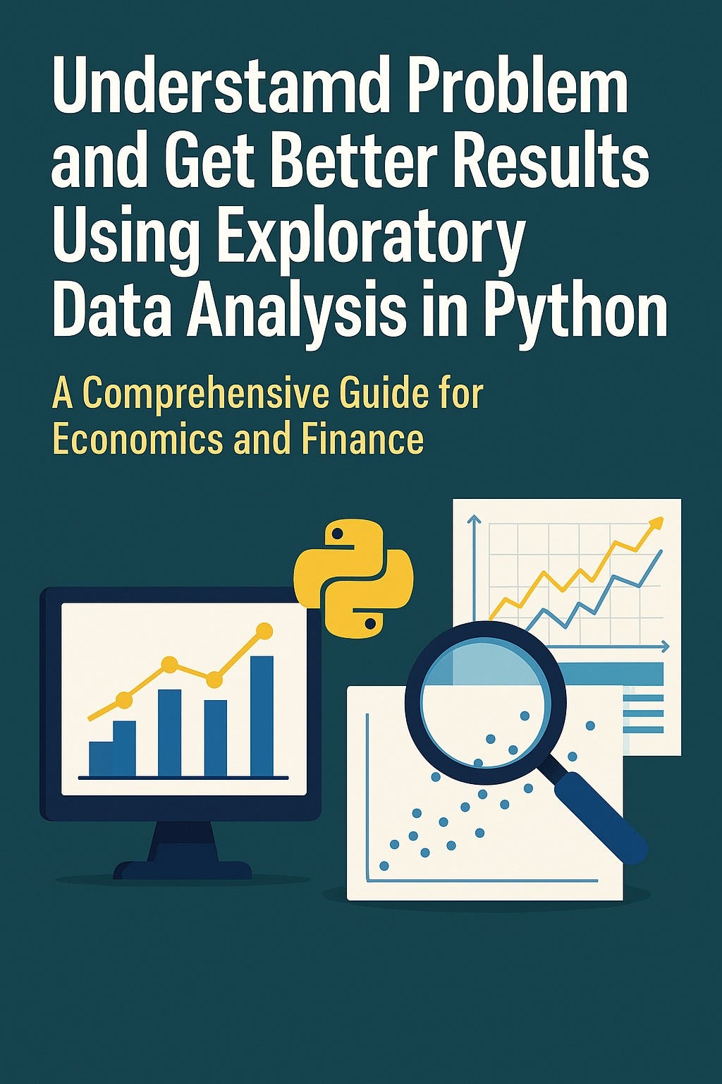
This article explains how systematic Exploratory Data Analysis with Python enables economists and financial analysts to uncover structure, spot issues, and develop stronger insights, laying the foundation for reliable economic and financial analysis.

Download the article … …. …

[embed]Understand Problem and Get Better Results Using Exploratory Data Analysis in Python: A… This article explains how systematic Exploratory Data Analysis with Python enables economists and financial analysts to…open.substack.com

Article Outline:

Introduction

• Why understanding your dataset and business question is essential in economics and finance.
• The critical role of Exploratory Data Analysis (EDA) in financial research, economic modeling, and data-driven decision-making.
• How Python empowers financial analysts and economists to perform in-depth EDA efficiently.

The Value of EDA in Economics and Finance

• Clarifying objectives, assumptions, and problem structure before modeling.
• Detecting data quality issues, outliers, anomalies, and patterns specific to economic and financial data.
• Supporting robust forecasting, investment analysis, and policy research with deep data insights.

Preparing and Importing Financial and Economic Data for EDA in Python

• Loading and organizing typical economics and finance datasets (e.g., time series, cross-sectional, panel data).
• Handling missing values, date/time columns, categorical and continuous features.
• Inspecting the initial structure and statistical summary of the dataset.

Core EDA Techniques and Visualisations in Finance and Economics

• Computing summary statistics: mean, median, volatility, percentiles, and skewness.
• Creating and interpreting line plots, histograms, boxplots, scatterplots, and correlation heatmaps for financial time series and economic variables.
• Segmenting and comparing groups (e.g., by sector, country, period) in financial or macroeconomic data.

End-to-End EDA Example in Python: Financial and Economic Dataset

• Simulating a dataset of stock returns, macroeconomic indicators, and company fundamentals.
• Workflow: initial checks, cleaning, univariate and bivariate analysis, visualisations, group and time-based exploration.
• Using pandas, matplotlib, and seaborn for analysis and visualization.
• Drawing practical insights and forming hypotheses for further modeling.

Best Practices and Common Pitfalls in EDA for Economics and Finance

• Ensuring reproducibility and documentation of EDA steps.
• Combining financial and economic domain expertise with statistical exploration.
• Avoiding common mistakes: overfitting, ignoring time dependencies, or misinterpreting spurious relationships.

Conclusion

• Summarising the benefits of EDA for clearer understanding and better decision-making in economics and finance.
• Encouragement to make EDA a standard, early practice in all financial and economic analytics projects.

End-to-End Python Example: EDA Workflow for Economics and Finance

## End-to-End Python Example: EDA Workflow for Economics and Finance

import warnings
warnings.filterwarnings("ignore")

import numpy as np
import pandas as pd
import matplotlib.pyplot as plt
import seaborn as sns

np.random.seed(100)
n_companies = 20
n_years = 8
sectors = ['Technology', 'Finance', 'Consumer', 'Industrial']
years = np.arange(2015, 2015 + n_years)

records = []
for company_id in range(1, n_companies + 1):
    sector = np.random.choice(sectors)
    base_return = np.random.normal(0.08, 0.04)
    volatility = np.random.uniform(0.10, 0.35)
    for year in years:
        gdp_growth = np.random.normal(2.2, 1.0)
        interest_rate = np.random.normal(2.0, 0.7)
        inflation = np.random.normal(1.8, 0.5)
        earnings_yield = np.random.normal(0.07, 0.02)
        price_to_book = np.random.normal(2.1, 0.6)
        return_ = (base_return +
                  0.004 * gdp_growth -
                  0.002 * interest_rate -
                  0.003 * inflation +
                  0.03 * (earnings_yield - 0.07) +
                  np.random.normal(0, volatility))
        # Random missing and outlier values
        if np.random.rand() < 0.03:
            return_ = np.nan
        if np.random.rand() < 0.03:
            return_ += np.random.choice([-0.18, 0.22])
        records.append({
            'company_id': company_id,
            'sector': sector,
            'year': year,
            'gdp_growth': gdp_growth,
            'interest_rate': interest_rate,
            'inflation': inflation,
            'earnings_yield': earnings_yield,
            'price_to_book': price_to_book,
            'annual_return': return_
        })

df = pd.DataFrame(records)

# Initial inspection
print(df.info())
print(df.isnull().sum())
print(df.describe())
print(df['sector'].value_counts())

# Clean for EDA: drop missing returns
df_clean = df.dropna(subset=['annual_return']).copy()

# Univariate
sns.histplot(df_clean['annual_return'], bins=20, kde=True, color='dodgerblue')
plt.title('Annual Return Distribution')
plt.show()

sns.boxplot(x='sector', y='annual_return', data=df_clean)
plt.title('Returns by Sector')
plt.show()

# Bivariate
sns.scatterplot(x='earnings_yield', y='annual_return', hue='sector', data=df_clean)
plt.title('Annual Return vs Earnings Yield')
plt.show()

sns.scatterplot(x='gdp_growth', y='annual_return', hue='sector', data=df_clean)
plt.title('Annual Return vs GDP Growth')
plt.show()

# Correlation matrix and heatmap
corr = df_clean[['annual_return', 'earnings_yield', 'price_to_book', 'gdp_growth', 'interest_rate', 'inflation']].corr()
print(corr)
sns.heatmap(corr, annot=True, cmap='vlag', fmt=".2f")
plt.title('Correlation Matrix')
plt.show()

# Grouped analysis
sector_summary = df_clean.groupby('sector').agg({
    'annual_return': ['mean', 'std', 'count'],
    'earnings_yield': 'mean',
    'price_to_book': 'mean'
})
print(sector_summary)

sector_year = df_clean.groupby(['sector', 'year'])['annual_return'].mean().reset_index()
sns.lineplot(x='year', y='annual_return', hue='sector', data=sector_year, marker='o')
plt.title('Sector Mean Returns Over Time')
plt.show()

# Outlier detection
Q1 = df_clean['annual_return'].quantile(0.25)
Q3 = df_clean['annual_return'].quantile(0.75)
IQR = Q3 - Q1

outliers = df_clean[(df_clean['annual_return'] < Q1 - 1.5 * IQR) | (df_clean['annual_return'] > Q3 + 1.5 * IQR)]
print("Potential outliers:\n", outliers[['company_id', 'sector', 'year', 'annual_return']])