One-Way ANOVA Test with RStudio

ANOVA (Analysis of Variance) is a statistical test to determine whether the means of two or more populations differ. In other words, it is used to compare two or more groups to see if they differ significantly.

To choose ANOVA as the appropriate test statistic, you must follow the steps in the flow chart below.

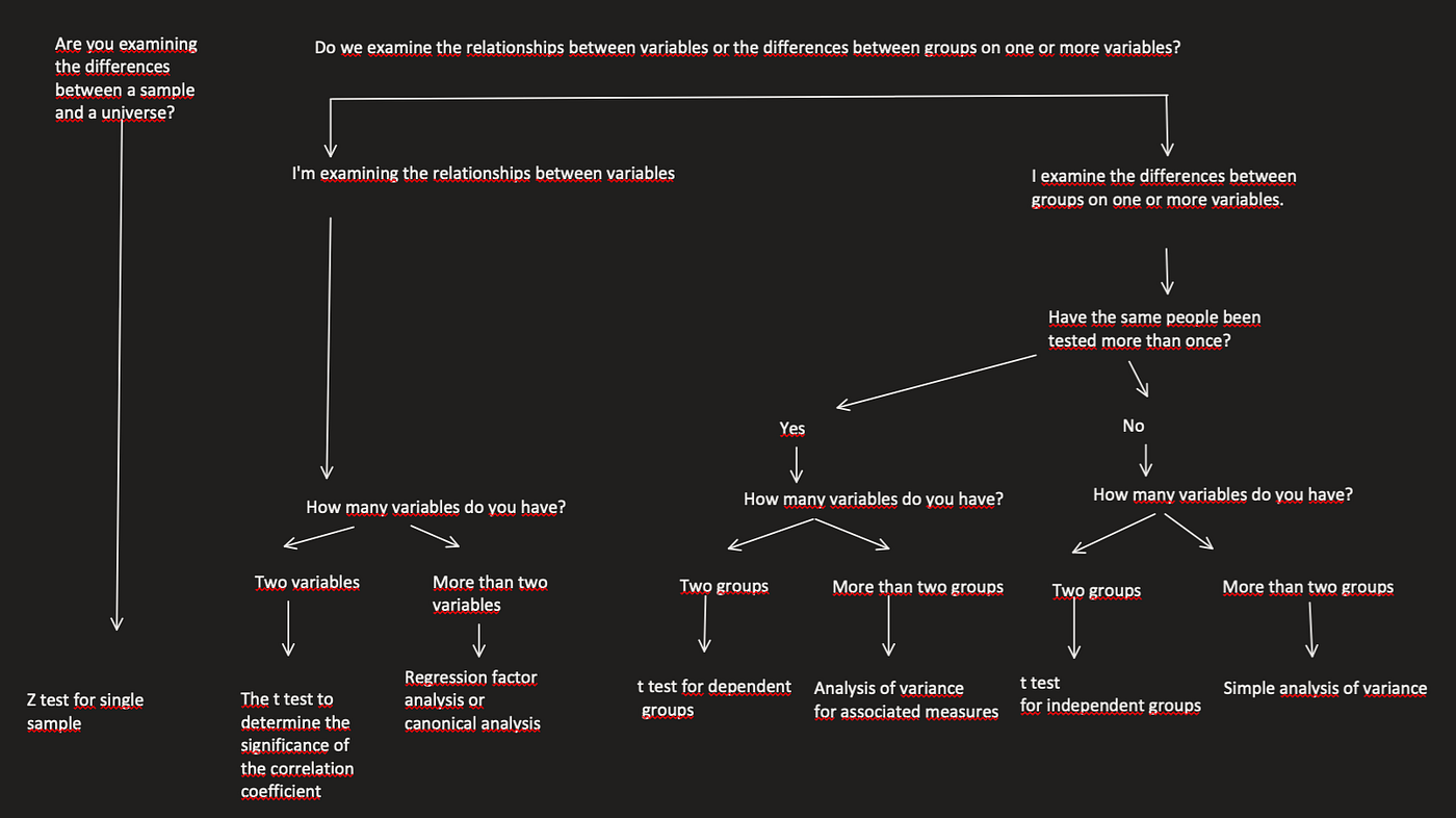
ANOVA Test

One-way ANOVA: an extension of the independent samples t-test to compare means in a situation where there are more than two groups. This is the simplest case of ANOVA testing, where data is organized into several groups based on just a single grouping variable (also called a factor variable).

There are several versions of ANOVA (one-way ANOVA, two-way ANOVA, mixed ANOVA, repeated-measures ANOVA, etc.). In this article, we only touch on one-way ANOVA.

In fact, ANOVA is similar to the t-test in many ways. In both methods, the differences between the means are calculated. But in ANOVA, the average number is more than two.

For example, let’s say we are investigating the effect of attending kindergarten for 5, 10, or 20 hours a week on language development. The group to which the children belong is the independent variable or group factor. Language development is the dependent variable that we measure. The experimental design with a three-level single variable (participation time) is as follows.

Assumptions

• Independence of observations: Each subject should belong to only one group. There is no correlation between the observations in each group. Repeated measurements for the same participants are not allowed.
• Outliers: No significant outliers in any cell of the design.
• Normality: The distribution of the data should be in the normal distribution.
• Homogeneity of variances: The variance of the outcome variable should be equal in every cell of the design.

If the above assumptions are not met, a non-parametric alternative Kruskal-Wallis test should be used based on one-way ANOVA.

Unfortunately, there are no non-parametric alternatives to two-way and three-way ANOVA. Therefore, if the assumptions are not met, you might consider running a two-way/three-way ANOVA on the transformed and untransformed data to see if there are significant differences.

Let’s create the data you see below in RStudio to see how to calculate the F value. For our example, suppose the data are language scores of three groups of kindergarten students.

# Libraries
library(tidyverse) # for data manipulation and visualization
library(ggpubr) # or creating easily publication ready plots
library(rstatix) # provides pipe-friendly R functions for easy statistical analyses

Let’s create data consisting of 3 groups.

# Data generation
set.seed(111) # if you want to get the same results, you must write the same set seed.
language_scores <- sample(x = 60:100, size = 30, replace = TRUE) # Get a distribution between 60 and 100 points with 30 observation

groups <- c(rep("first_grup", 10),
         rep("second_grup", 10),
         rep("third_grup", 10))

simple_data = data.frame(groups, language_scores) # to make the series dataframe
str(simple_data)

Now let’s calculate the F test statistic by following the steps below.

Statement of research hypothesis and null hypothesis.

The null hypothesis states that there is no difference between the means of these three different groups. AVOVA, sometimes called the F test (as it produces an F statistic or an F ratio), generally looks for differences between groups.

The F test does not look for pairwise differences, such as the difference between Group 1 and Group 2. For this we need to use another method.

The research hypothesis is; means that the averages are different from each other. Notice that the direction for the differences is not specified because all F tests are non-directional.

There are no single- and double-tailed tests for ANOVA. Because more than two groups are tested and group differences are looked at collectively (it is not said which two groups differ), it is meaningless to talk about the direction of individual differences.

1. Descriptive Statistics

simple_data %>%
  group_by(groups) %>%
  get_summary_stats(language_scores, type = "mean_sd")

2. Visualization

ggboxplot(simple_data, x = "groups", y = "language_scores")

3. Assumptions

3.1 Outliers

Outliers can be easily identified using box drawing methods with the define_outliers() function in the rstatix package.

simple_data %>% 
  group_by(groups) %>%
  identify_outliers(language_scores)

There is no outlier value.

3.2 Normality Assumption The normality assumption can be checked using one of the following two approaches:

1. It involves analyzing ANOVA model residues together to check for normality for all groups. This approach is easier and is very useful when you have many groups or several data points (observations) per group.

2. Check for normality separately for each group. This approach can be used when you only have a few groups and many data points (observations) per group.

Let’s do both option 1 and option 2.

Check the normality assumption by analyzing the model residuals. QQ chart and Shapiro-Wilk normality test were used. The QQ chart plots the correlation between a given data and the normal distribution.

# FIRST OPTION
# Build the linear model
model  <- lm(language_scores ~ groups, data = simple_data)
# Create a QQ plot of residuals
ggqqplot(residuals(model))

# Shapiro-Wilk normality test
shapiro_test(residuals(model))

In the QQ plot, we can assume normality as all points fall approximately along the reference line. This result is supported by the Shapiro-Wilk test. The p-value is not significant (p = 0.45), so we can assume normality.

We check the assumption of normality by groups. Calculation of the Shapiro-Wilk test for each group level. If the data are normally distributed, the p-value should be greater than 0.05.

simple_data %>%
  group_by(groups) %>%
  shapiro_test(language_scores)

It was normally distributed for each group as assessed by Shapiro-Wilk’s test of normality (p > 0.05).

Note that if your sample size is larger than 50, the normal QQ plot is preferred because at larger sample sizes the Shapiro-Wilk test becomes very sensitive to even a small deviation from normality.

The QQ chart plots the correlation between a given data and the normal distribution. Create QQ charts for each group level:

ggqqplot(simple_data, "language_scores", facet.by = "groups")

All points are located approximately along the reference line for each cell. Thus, we can assume that the data are normally distributed.

Note: If you are in doubt about the normality of the data, you can use the Kruskal-Wallis test, which is a non-parametric alternative to the one-way ANOVA test.

Homogeneity of Variance¶

1. The residuals-fit plot can be used to check the homogeneity of the variances.

plot(model, 1)

In the graph above, there is no obvious relationship between residuals and fit values (mean of each group), which is fine. So we can assume homogeneity of variances.

It is also possible to use the Levene test to check for homogeneity of variances:

From the above output we can see that the p-value is > 0.05, which is not significant. This means that there is no significant difference in variances between groups. Therefore, group variance homogeneity is also ensured.

In a situation where the variance homogeneity assumption is not met, you can use the Welch one-way ANOVA test using the welch_anova_test()[rstatix package] function. This test does not require the equal variance assumption.

res.aov <- simple_data %>% anova_test(language_scores ~ groups)
res.aov

Since the p value is greater than p > 0.05, it is seen that there is no significant difference between the groups.

In the table above, the ges column corresponds to the generalized eta square, that is, the effect size. It measures the proportion of variability in the outcome variable (language score) that can be explained in terms of the predictor (group). An effect size of 0.18 (18%) means that 18% of the variation in weight can be explained for the language score.

References

• https://statsandr.com/blog/anova-in-r/
• https://www.datanovia.com/en/lessons/anova-in-r/
• İstatistikten Nefret Edenler İçin İstatistik — Neil Salkind