Don’t Run Today’s Trades Without These 7 Pandas Moves — Part 1
This is part one of my three part series on using Python + Pandas for real trading and investing workflows, and there is a bonus content…
Don’t Run Today’s Trades Without These 7 Pandas Moves — Part 1
This is part one of my three part series on using Python + Pandas for real trading and investing workflows, and there is a bonus content at the end to solve one of the big issues that we all have with Yahoo Finance since the start of 2025.
Source of image
Table of Contents:
- **Why I Wrote This.**
- **Step 1: Load Some Real Market Data.**
- **Step 2: Calculate Daily Returns.**
- **Step 3: Deal with Missing Data.**
- **Step 4: Compare Two Stocks Side by Side.**
- **Step 5: Spot the High-Volatility Days.**
- **Step 6: Create a Simple Trend Indicator.**
- **Step 7: Label Bull, Neutral, and Bear Regimes.**
- **ELI5: How the 20-Day Cumulative Return Bucket Works.**
- **What You’ve Learned So Far.**
- **One Practical Use Case: Filter Trades on Volatile Days.**
- **Bonus Content: There is a big issue now with Yahoo Finance.**
- **What’s Next in Part 2: Strategy and Portfolio Logic**
- **Conclusion.**
Why I Wrote This
A few years ago, I built my first trading strategy in Excel. It worked, sort of — until it didn’t. Formulas would break. Data would go missing. The whole thing felt fragile. So I switched to Python. Pandas was the tool everyone talked about. But when I tried to use it for actual trading logic — moving averages, backtests, volatility filters — I hit a wall. The syntax was weird. Most tutorials used fake data. And no one explained how real traders actually think. This series is my attempt to fix that. You’ll be working with real stock data, building logic to detect trends, label market regimes, and build reusable strategy tools that feel closer to how actual quants and algo traders operate. Let’s get into it.
Step 1: Load Some Real Market Data
We’ll use yfinance to pull Apple (AAPL) stock data — it’s free, reliable enough, and perfect for this kind of work.
!pip install curl_cffi yfinance pandasimport yfinance as yf
import pandas as pd
import time
aapl = yf.download("AAPL", session=session,start="2020-01-01", end="2024-01-01")
print(aapl.head)This gives you a tidy time-indexed DataFrame: open, high, low, close, volume. Close which is what we care about most. That column adjusts for dividends and stock splits, making it a better input for return-based analysis.
Step 2: Calculate Daily Returns
In finance, price is what you pay. But returns are what really matter.
aapl['Daily Return'] = aapl['Close'].pct_change()
aapl['Daily Return'].plot(title="AAPL Daily Returns")
This gives us the percentage change in price from one day to the next — the foundation of all performance, volatility, Sharpe ratios, and drawdown calculations. It’s also the raw material for every strategy you’ll ever build.
Step 3: Deal with Missing Data
Financial data has holes — holidays, outages, weird gaps from the data provider. Don’t let it break your backtest.
aapl['Close'].isna().sum()
aapl.iloc[5:10, aapl.columns.get_loc('Close')] = None
aapl['Close'].isna().sum()
aapl.iloc[4:11, aapl.columns.get_loc('Close')]
aapl['Close'] = aapl['Close'].fillna(method='ffill')
aapl.iloc[4:11, aapl.columns.get_loc('Close')]
This line keeps your strategy running even when there’s no new data. It’s not fancy, but in the real world, it’s necessary.
Step 4: Compare Two Stocks Side by Side
Want to see how Apple did vs Microsoft? Normalize both to $1 on day one:
msft = yf.download("MSFT", start="2020-01-01", end="2024-01-01")
combined = pd.DataFrame({
    'AAPL': aapl['Close']['AAPL'],
    'MSFT': msft['Close']['MSFT'],
})

normalized = combined / combined.iloc[0]
normalized.plot(title="AAPL vs MSFT (Normalized to $1)")
This shows how $1 invested in each company grew over time — a clean, intuitive way to compare performance.
Step 5: Spot the High-Volatility Days
Let’s say you’re building a risk model. You might want to skip trades on days when volatility is too high.
high_vol = aapl[aapl['Daily Return'].abs() > 0.021]
print(high_vol[['Close', 'Daily Return']].head())
Here, we’re filtering for days when Apple moved more than ±2%. You’d be surprised how often those days cluster around earnings reports or macro news. You can also use this to build “volatility filters” that pause your strategy when the market gets too jumpy.
Step 6: Create a Simple Trend Indicator
Let’s introduce one of the most classic technical indicators: the moving average.
close_series = aapl['Close']['AAPL']
aapl['20D MA'] = close_series.rolling(window=20).mean()
aapl['Trend Signal'] = (close_series > aapl['20D MA']).astype(int)
This Trend Signal column will be 1 when the price is above the 20-day moving average (bullish), and 0 when it’s below (bearish). It’s the backbone of hundreds of trend-following systems — from simple bots to hedge fund models.
Step 7: Label Bull, Neutral, and Bear Regimes
Let’s go a step further: use rolling returns to define whether the market is currently in a bull, neutral, or bear regime.
aapl['20D Cum Return'] = aapl['Daily Return'].rolling(window=20).sum()
aapl['Market Regime'] = pd.cut(
    aapl['20D Cum Return'],
    bins=[-1, -0.05, 0.05, 1],
    labels=['Bear', 'Neutral', 'Bull']
)
aapl[['Daily Return','20D Cum Return','Market Regime']].tail(11)
ELI5: How the 20-Day Cumulative Return Bucket Works
Now every day has a label. You can use this to change risk levels, switch strategies, or even just better visualize your backtests. For a more ELI5 explanation of the code read this please:
If over the last 20 days you had returns of +0.5%, +0.7%, –0.2%, … up to day 20, summing them gives you something like +8.3% total.
For dates before you have 20 days of history, you’ll see
NaNbecause there isn’t a full window yet.
Anything ≤ −5% (down 5% or more in 20 days) falls into the first bucket. If your 20-day cumlative return is −8%, it becomes bear.
Between −5% and +5% is considered neutral. If it’s +2%, it’s neutral.
Anything ≥ +5% is the bull bucket. If it’s +12%, that’s definitely bull territory.
What You’ve Learned So Far
What You Built Why It Matters Daily Returns Basis for any kind of trading strategy Fill Missing Data Avoid silent errors or broken pipelines Stock Comparisons Track relative performance over time Volatility Filter Avoid high-risk trades or events Moving Average Signal Momentum/trend entry-exit logic Regime Detection Dynamic strategy switching / allocation.
One Practical Use Case: Filter Trades on Volatile Days
Imagine you have a signal to buy AAPL. But you only want to enter when the market is “calm.”
Just use this:
signal = (aapl['Trend Signal'] == 1)
not_too_volatile = (aapl['Daily Return'].abs() < 0.021)
filtered_signal = signal & not_too_volatile
You’ve just created a strategy filter that only buys when the trend is up and volatility is manageable.
Bonus Content: There is a big issue now with Yahoo Finance.
import yfinance as yf
import pandas as pd
import time
from curl_cffi import requests

session = requests.Session(impersonate="chrome")
aapl = yf.download("AAPL", session=session,start="2020-01-01", end="2024-01-01")
msft = yf.download("MSFT", session=session,start="2020-01-01", end="2024-01-01")
print(aapl.head)
If you do it the old way, like you did in the first step you will have this error
YFRateLimitError('Too Many Requests')so in order to avoid the error you need to use curl_cffi package and use a session.
In Part 2: Strategy and Portfolio Logic
In Part 2, we’ll start putting these tools into motion:
- Resample daily data into monthly
- Build a simple moving average crossover strategy
- Simulate a 60/40 portfolio with SPY and AGG
- Measure Sharpe ratio and max drawdown
- Rank ETFs by momentum
Conclusion
If this article saved you an hour or two of Googling — or got you excited to build your own trading notebook — send it to a friend or give me a like. If you’d like me to turn all 3 parts into a downloadable notebook or GitHub repo, let me know in the comments below.
메타데이터
- post_id
- 490ea94ffaee
- slug
- dont-run-today-s-trades-without-these-7-pandas-moves-part-1-490ea94ffaee
- url
- https://medium.com/@dataakkadian/dont-run-today-s-trades-without-these-7-pandas-moves-part-1-490ea94ffaee
- canonical_url
- https://medium.com/@dataakkadian/dont-run-today-s-trades-without-these-7-pandas-moves-part-1-490ea94ffaee
- author_url
- https://medium.com/@dataakkadian
- status
- ok
- fetched_at
- 2026-07-30 18:47:05