Part XI: Vehicle Detection Using OpenCV and Deep Learning

[embed]Part X: Behavioral Cloning Using Deep Learning Behavioral cloning is a technique for identifying and reproducing human sub-cognitive abilities within a computer…medium.com

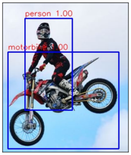
In self-driving cars, understanding object detection is crucial. Object detection involves both classifying objects and localizing them. In the following image, for example, a biker is detected as a person in a bounding box, and the bike is detected as a motorbike.

In this section, we will dive into YOLO and its architecture.

What makes YOLO different?

YOLO (You Only Look Once) was first developed in 2015 as a fast deep learning architecture for object detection. Over the years, it has undergone many updates, with different developers, and currently, it has reached its 11th version. YOLO stands out by using a single neural network that processes the image in one pass to make predictions, which makes it 1000 times faster than other object detection networks. This architecture treats detection as a regression problem, enabling quick and accurate results.

Here’s a summary of its methodology:

• YOLO takes the input image and divides it into an SxS grid, where each grid cell predicts an entity.
• For each entity, YOLO applies image classification and localization.
• Each grid cell is responsible for detecting an object if a part of the object falls within that cell.
• All grid cells predict bounding boxes with corresponding confidence scores.

The YOLO loss function

The YOLO loss function is calculated through the following steps:

1. First, we identify the bounding boxes with the highest Intersection over Union (IoU) with the ground truth bounding boxes.
2. We then calculate the confidence loss, which represents the probability that an object is present inside a given bounding box.
3. Next, we compute the classification loss, which indicates the predicted class of objects within the bounding box.
4. Finally, we calculate the coordinate loss to match the positions of the detected boxes with the ground truth.

In formulaic terms, the YOLO loss function is the sum of the coordinate loss, classification loss, and confidence loss.

The YOLO architecture

The YOLO architecture is inspired by the image classification model created by GoogLeNet. The network consists of 24 convolutional layers followed by two fully connected layers. It also incorporates alternating 1x1 convolutional layers, which are used to reduce the feature space from preceding layers.

The convolutional layers in YOLO are based on a pre-trained model from the ImageNet task, sampled initially at a half resolution (224x224) and then at double resolution. YOLO applies a leaky ReLU activation function to all layers, with a linear activation function used in the final layer. The following figure provides an overview of this architecture.

Fast YOLO

Fast YOLO is a faster version of the original YOLO model. It uses 9 convolutional layers and fewer filters compared to YOLO, which reduces computational complexity. The training and testing parameters are the same for both models. The output of Fast YOLO is a 7x7x30 tensors.

YOLO v2

YOLO v2, also known as YOLO9000, increases the input size from 224x224 to 448x448. This increase in resolution has been observed to improve performance, resulting in a higher mean Average Precision (mAP). YOLO v2 also uses batch normalization, which significantly improves model accuracy. Additionally, this model performs better at detecting small objects compared to the previous version. In the following figure, you can see the anchor boxes used by YOLO v2 for quick and accurate classification.

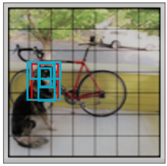
In this picture, the blue boxes are anchor boxes, and the red box represents the ground truth box for the object. YOLO v2 uses the DarkNET architecture for object classification, consisting of 19 convolutional layers, five max-pooling layers, and a softmax layer.

YOLO v3

YOLOv3 is one of the most popular YOLO models. It uses 9 anchor boxes and employs logistic regression for predictions instead of softmax. Additionally, YOLOv3 uses the Darknet-53 network for feature extraction, which consists of 53 convolutional layers.

Implementation of YOLO object detection

We now have a basic understanding of YOLO and its architecture. Next, we will implement it using the COCO dataset. This dataset contains 1.5 million object instances across 80 different object categories. We will use a pre-trained model, but if you want to train your own model, you can refer to my paper on this topic. However, training requires a labeled dataset and a powerful machine, or you can use platforms like Roboflow.

Now, let’s introduce the COCO model. COCO stands for Common Objects in Context, and it is a large-scale dataset for object detection, segmentation, and captioning.

The COCO dataset includes:

• 250,000 people with keypoints
• 330k images, with over 200k labeled
• 1.5 million object instances
• 80 object categories
• 91 stuff categories
• Object segmentation
• Recognition in context
• Superpixel stuff segmentation

Let’s start by downloading the “yolov3.weights” and “yolov3.cfg” files. You can find them by searching on Google.

Detecting objects in images

import cv2
import numpy as np
import matplotlib.pyplot as plt

# Load YOLOv3 weights and configuration file
net = cv2.dnn.readNet("yolov3.weights", "yolov3.cfg")

# Load class names from the coco.names file
with open("coco.names", "r") as f:
    classes = [line.strip() for line in f.readlines()]

# Load image
img = cv2.imread("bus.jpg")
if img is None:
    print("Error: Image not found or unable to load.")
else:
    height, width, channels = img.shape

    # Convert BGR image to RGB for displaying with matplotlib
    img_rgb = cv2.cvtColor(img, cv2.COLOR_BGR2RGB)

    # Create a blob for YOLO input
    blob = cv2.dnn.blobFromImage(img, 0.00392, (416, 416), (0, 0, 0), True, crop=False)

    # Set the input to the network
    net.setInput(blob)

    # Get the names of all layers
    layer_names = net.getLayerNames()

    # Output layers are the final layers (i.e., "output" layers)
    output_layers = [layer_names[i - 1] for i in net.getUnconnectedOutLayers()]

    # Perform a forward pass through the network
    outs = net.forward(output_layers)

    # Process the detection results
    class_ids = []
    confidences = []
    boxes = []
    for out in outs:
        for detection in out:
            scores = detection[5:]
            class_id = np.argmax(scores)
            confidence = scores[class_id]
            if confidence > 0.5:  # Confidence threshold
                center_x = int(detection[0] * width)
                center_y = int(detection[1] * height)
                w = int(detection[2] * width)
                h = int(detection[3] * height)
                x = center_x - w // 2
                y = center_y - h // 2
                boxes.append([x, y, w, h])
                confidences.append(float(confidence))
                class_ids.append(class_id)

    # Apply non-maxima suppression to remove redundant boxes
    indices = cv2.dnn.NMSBoxes(boxes, confidences, 0.5, 0.4)

    # Display the detected objects
    for i in indices.flatten():
        x, y, w, h = boxes[i]
        label = str(classes[class_ids[i]])
        cv2.rectangle(img, (x, y), (x + w, y + h), (0, 255, 0), 2)
        cv2.putText(img, label, (x, y - 10), cv2.FONT_HERSHEY_SIMPLEX, 0.5, (0, 255, 0), 2)

    # Convert the image to RGB for plotting
    img_rgb = cv2.cvtColor(img, cv2.COLOR_BGR2RGB)

    # Use matplotlib to show the image
    plt.figure(figsize=(8,8))
    plt.imshow(img_rgb)
    plt.axis('off')  
    plt.show()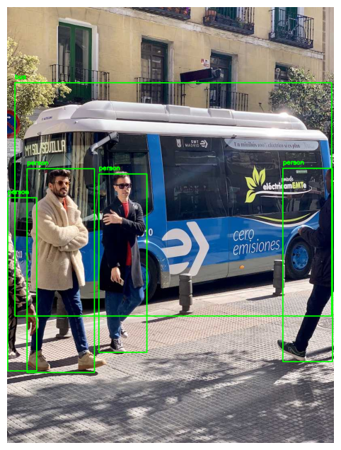

Detect video function

Similar to the image function, this function helps work with videos.

import cv2
import numpy as np

# Load YOLOv3 weights and configuration file
net = cv2.dnn.readNet("yolov3.weights", "yolov3.cfg")

# Load class names from the coco.names file
with open("coco.names", "r") as f:
    classes = [line.strip() for line in f.readlines()]

# Load the video
cap = cv2.VideoCapture("traffic13.mp4")

# Get video properties for output video
frame_width = int(cap.get(cv2.CAP_PROP_FRAME_WIDTH))
frame_height = int(cap.get(cv2.CAP_PROP_FRAME_HEIGHT))
fps = cap.get(cv2.CAP_PROP_FPS)

# Define codec and create VideoWriter object to save the processed video
out = cv2.VideoWriter("output_video.mp4", cv2.VideoWriter_fourcc(*'mp4v'), fps, (frame_width, frame_height))

while cap.isOpened():
    ret, frame = cap.read()  # Read a frame from the video
    if not ret:
        break  # If no frame is returned, exit the loop

    # Prepare the frame for YOLO detection
    blob = cv2.dnn.blobFromImage(frame, 0.00392, (416, 416), (0, 0, 0), True, crop=False)
    net.setInput(blob)
    output_layers = net.getUnconnectedOutLayersNames()
    detections = net.forward(output_layers)

    # Process detections
    class_ids = []
    confidences = []
    boxes = []

    for detection in detections:
        for obj in detection:
            scores = obj[5:]
            class_id = np.argmax(scores)  # Get class ID with the highest score
            confidence = scores[class_id]  # Get the confidence score
            if confidence > 0.5:  # Filter out weak detections
                center_x = int(obj[0] * frame.shape[1])
                center_y = int(obj[1] * frame.shape[0])
                w = int(obj[2] * frame.shape[1])
                h = int(obj[3] * frame.shape[0])

                # Rectangle coordinates
                x = int(center_x - w / 2)
                y = int(center_y - h / 2)

                boxes.append([x, y, w, h])  # Store the bounding box
                confidences.append(float(confidence))
                class_ids.append(class_id)

    # Apply non-maxima suppression to remove overlapping boxes
    indices = cv2.dnn.NMSBoxes(boxes, confidences, 0.5, 0.4)

    # Draw bounding boxes and class labels on the frame
    if len(indices) > 0:
        for i in indices.flatten():
            x, y, w, h = boxes[i]
            label = str(classes[class_ids[i]])  # Class label
            color = (0, 255, 0)  # Green color for bounding box
            cv2.rectangle(frame, (x, y), (x + w, y + h), color, 2)
            cv2.putText(frame, label, (x, y - 10), cv2.FONT_HERSHEY_SIMPLEX, 0.5, color, 2)

    # Write the processed frame to the output video
    out.write(frame)

# Release resources
cap.release()
out.release()

print("Video processing complete. Output saved as 'output_video.mp4'.")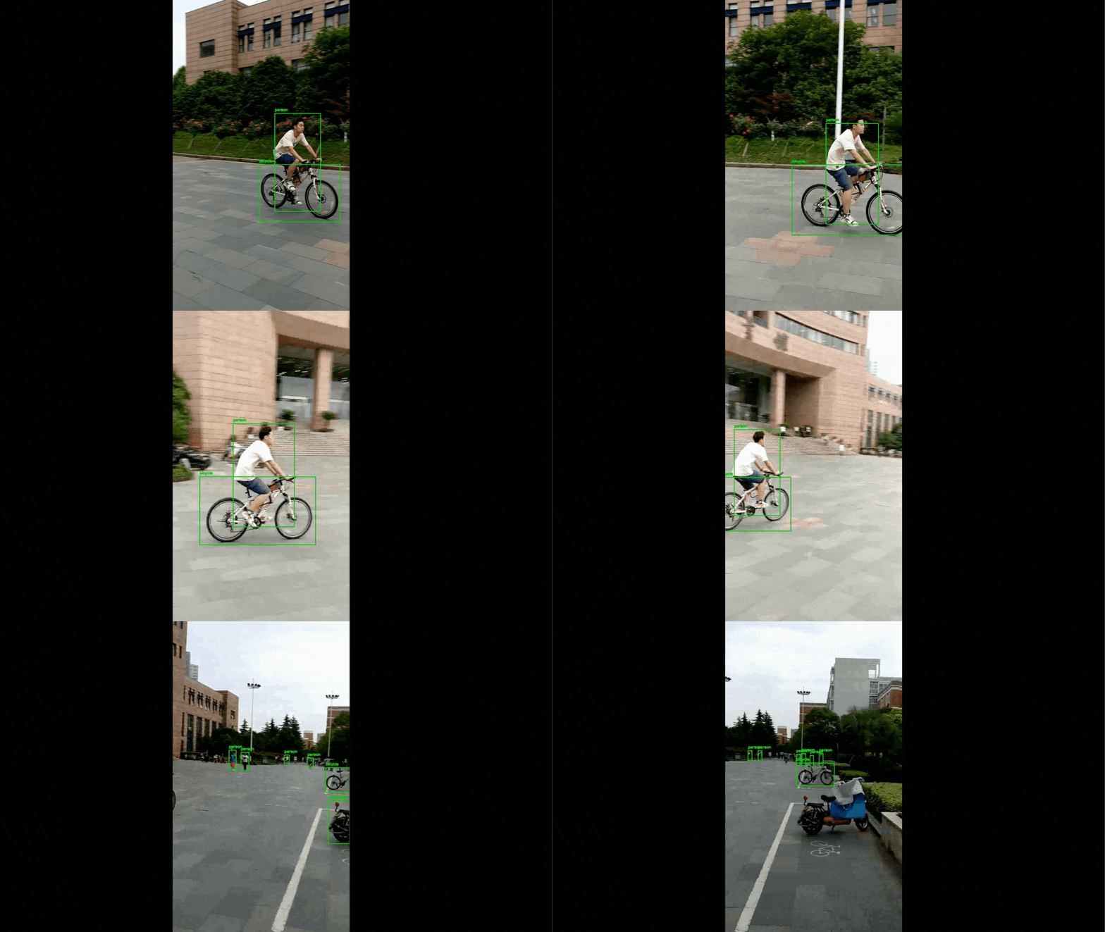

[embed]GitHub - muhammeddincmdx/Sdcs-Part11 Contribute to muhammeddincmdx/Sdcs-Part11 development by creating an account on GitHub.github.com

Note: End of the Part VI.