Solving the Schrödinger Equation with PyTorch: A Guide to Quantum PINNs

If you work in Machine Learning, you are used to the standard paradigm: gather a massive dataset (X_train, y_train), feed it into a neural network, and calculate the loss between the predictions and the labels. But what if you have no data?

What if, instead of giving the AI the answers, you only gave it the laws of physics?

This is the premise of a Physics-Informed Neural Network (PINN). Instead of learning from a CSV file, the network learns by minimizing a loss function based on differential equations. In this article, I’ll walk through how I used PyTorch to build a PINN that solves the 1D Schrödinger equation from scratch, discovering the ground state (E1) and the first excited state (E2) of a quantum particle in a box.

1. The Problem: A Particle in a 1D Box

Imagine a quantum particle trapped in a 1D box of length L=1. The walls are infinitely high, meaning the particle cannot exist outside the box.

We need to find two things:

The Wavefunction (ψ): The curve that describes the probability of finding the particle at a given point x.

The Energy (E): The specific energy levels the particle is allowed to have.

The governing law here is the time-independent Schrödinger Equation (using atomic units where ℏ=1,m=1):

2. The Neural Network setup

Standard neural networks output predictions based on weights and biases. But we also need the network to find the Energy (E). PyTorch has a brilliant feature for this: nn.Parameter.

We can define E as a trainable parameter, meaning PyTorch will update E alongside the network weights during backpropagation!

class QuantumPINN(nn.Module):
    def __init__(self):
        super().__init__()
        # Use Tanh, not ReLU! ReLU's second derivative is 0, which breaks PDEs.
        self.net = nn.Sequential(
            nn.Linear(1, 64), nn.Tanh(),
            nn.Linear(64, 64), nn.Tanh(),
            nn.Linear(64, 1)
        )
        # The Energy eigenvalue (E) - initialized at a random guess
        self.E = nn.Parameter(torch.tensor([1.0], requires_grad=True))

    def forward(self, x):
        return self.net(x)

3. Training Without Data: The Custom Loss Function

Instead of Mean Squared Error against a dataset, our loss function is made of three physical rules:

Boundary Loss: The wavefunction must be exactly 0 at the walls (x = 0 and x = 1).

PDE Loss: The network’s output must satisfy the Schrödinger equation. We use torch.autograd to literally calculate the exact second derivative of the network’s output with respect to the input!

Normalization Loss: The total probability of finding the particle somewhere must be 1.

4. The First Trap: The Trivial Solution Collapse

When I first ran this code, my loss dropped beautifully, and the Energy settled around 4.93. But suddenly, at epoch 2500, the network completely collapsed. The loss spiked and locked forever.

What happened? The AI found a loophole. The neural network realized that if it just outputs exactly 0.0 everywhere, the Boundary loss is 0, and the derivative is 0 (PDE loss = 0). It flattened the wavefunction completely, deleting the particle from existence just to make the math easier!

The Fix: I had to heavily weight the Normalization loss (100.0 loss_norm*) to penalize the network for outputting zeros. Once balanced, the network converged beautifully.

The Result: The network found E1 = 4.932 . The analytical mathematical answer is :

The AI discovered quantum mechanics purely through calculus!

5. Climbing the Quantum Ladder: Finding E2

Finding the ground state was amazing, but I wanted the second state (n=2). Standard ML optimizers like Adam are “lazy” — they will always roll down the hill to the easiest solution (the ground state).

To force the AI to find E2, I had to introduce a new rule: Orthogonality.

The second state must have zero mathematical overlap with the first state. I froze the ground state model and trained a second model alongside it, adding an overlap penalty to the loss function.

The Second Trap: Reward Hacking Once again, the AI tried to outsmart me. I put a massive weight on the Orthogonality loss to force it away from the ground state. The AI looked at the massive penalty, looked at the math, and decided to just output 0.0 again. It accepted a flat loss of 10.0 because doing the hard physics was “too expensive” for the optimizer!

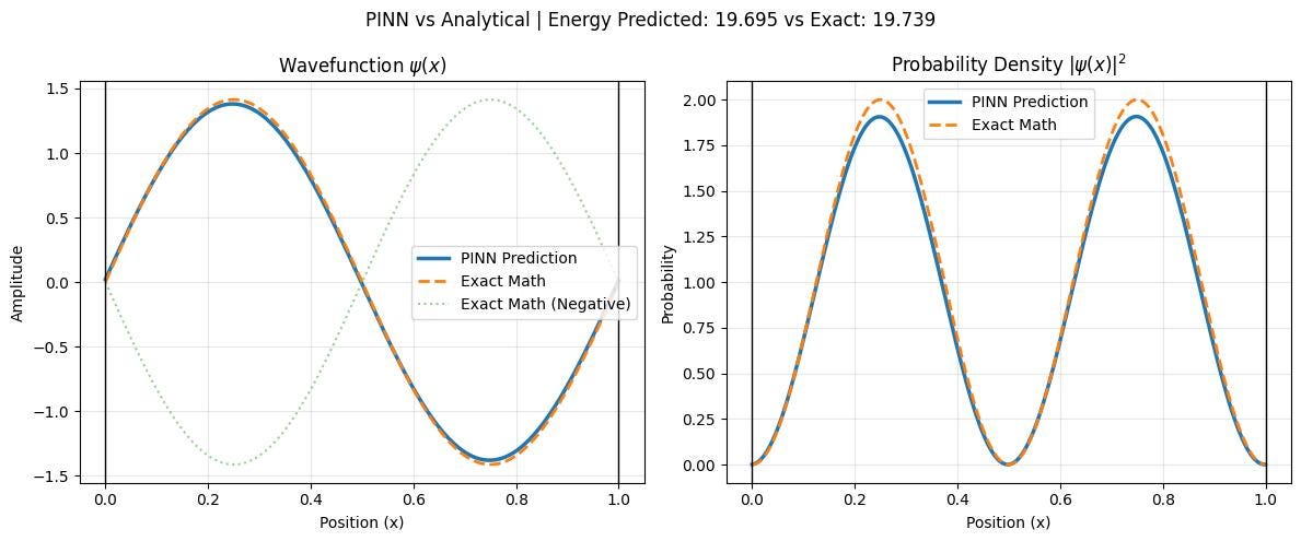
After rebalancing the weights so that Normalization was strictly the highest priority, the model was forced to bend the curve into a full sine wave.

The Final Result: The model converged to E2 = 19.74 ​

Conclusion

Building a PINN requires a fundamental shift in how you think about machine learning. You are no longer fitting curves to data; you are sculpting loss landscapes using the rules of the universe.

Watching a neural network deduce the energy states of a quantum system with zero training data feels like magic. If you are a standard data-driven ML practitioner, I highly recommend trying out PINNs — just be prepared for the AI to try and cheat the laws of physics along the way.