Building a Field-Oriented Control (FOC) Simulator with LTspice and Python, with AI-Assisted Controller Tuning

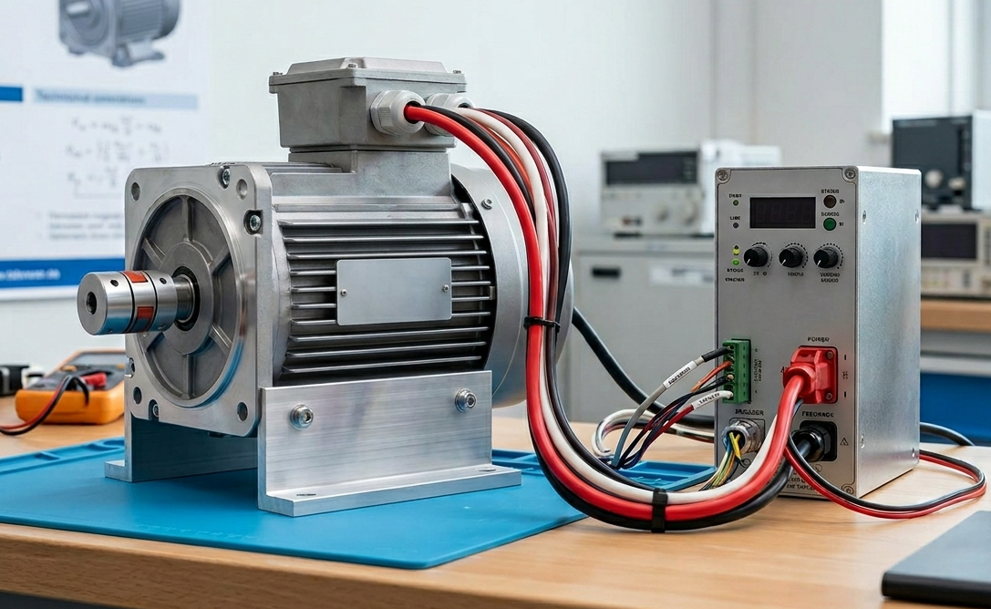
Field-Oriented Control (FOC) has become the de-facto standard for controlling Permanent Magnet Synchronous Motors (PMSM) and Brushless DC (BLDC) motors in applications ranging from drones and electric vehicles to industrial automation and robotics.

Most educational examples of FOC focus on the control theory itself and implement both the motor model and the controller inside the same simulation environment, typically MATLAB/Simulink. While this approach is excellent for understanding the mathematics, it often hides the realities of the electrical system behind simplified motor equations.

For this project, I wanted a different approach.

And, as I always say if you’re too hurry to take a look to the source code go to the following link: https://github.com/pablojoaquim/FOC-PMSM-ControlLab

Rather than simulating both the controller and the plant inside a single framework, I built a co-simulation environment where:

• LTspice simulates the physical motor and power stage.
• Python executes the Field-Oriented Control algorithm.
• Both systems exchange signals during simulation!

The result is a simulation architecture that is much closer to what happens in a real embedded motor control application.

Why Use LTspice for Motor Simulation?

When engineers think about motor control simulation, LTspice is usually not the first tool that comes to mind. MATLAB, Simulink, PSIM are far more common choices.

However, LTspice offers several advantages:

• Accurate Electrical Simulation: LTspice solves the circuit using SPICE numerical methods, providing detailed visibility into
• Phase currents
• Switching transients
• PWM ripple
• Power stage dynamics
• Voltage saturation effects
• Free and Widely Available: LTspice is widely used in power electronics design and is freely available. This makes the entire simulation environment reproducible without requiring expensive licenses.
• Easy Integration with Python: Using PyLTSpice and related automation tools, simulations can be launched, configured, and analyzed directly from Python.
• AI-Agent tuning: Rather than relying on traditional trial-and-error tuning, the agent explored the controller parameter space automatically and converged toward a gain set that satisfied the desired performance criteria.

This opens the door to hybrid simulation architectures where control algorithms and circuit simulations coexist.

System Architecture

The simulator is built around a clear separation between the physical plant and the digital controller, closely mirroring the architecture of a real motor control system.

Rather than implementing both the motor and the controller inside a single simulation environment, the project uses two specialized tools working together:

• LTspice models the electrical and mechanical behavior of the motor drive system.
• Python executes the Field-Oriented Control (FOC) algorithm.

This separation allows the controller to interact with the motor exactly as it would in a real embedded application, through measured currents and rotor position feedback rather than direct access to internal motor equations.

LTspice as the Physical Plant

The LTspice portion of the simulation represents the hardware side of the system.

During each simulation step, LTspice computes the electrical response of the motor and provides the same feedback signals that would be available on a real system:

• Phase currents Ia​, Ib​, and Ic
• Rotor electrical position θ​

These measurements are then passed to the controller, which treats them as sensor data.

Because LTspice solves the underlying circuit equations directly, the resulting current waveforms naturally include the electrical dynamics of the motor and inverter, providing a significantly more realistic plant model than the simplified transfer functions commonly found in educational examples.

Python as the Digital Controller

The control layer is implemented entirely in Python and contains the complete FOC algorithm.

At every control cycle, the controller receives the measured phase currents and rotor position from LTspice and processes them through the standard vector-control pipeline:

1. Clarke transformation
2. Park transformation
3. D-axis current regulation
4. Q-axis current regulation
5. Inverse Park transformation
6. Inverse Clarke transformation

The output of this process is a new set of three-phase voltage commands Va, Vb​, and Vc​, which are applied back to the LTspice model.

From the controller’s perspective, the motor is a black box. It has no knowledge of winding resistance, inductance, back-EMF equations, or mechanical parameters. It only sees sensor measurements and reacts accordingly, exactly like firmware running on a microcontroller. This separation makes the controller portable and allows future migration to actual hardware with minimal changes.

Understanding the FOC

FOC is based on a simple idea: Rather than controlling three sinusoidal currents independently, transform them into a rotating reference frame where they appear as DC quantities. This dramatically simplifies control!

Controlling a PMSM appears complicated because the controller must manage three independent phase currents:

Fortunately, in a balanced three-phase machine these currents are not independent. At every instant, their sum is equal to zero:

This means that only two degrees of freedom actually exist. The purpose of Field-Oriented Control is to exploit this property and transform the three-phase system into a representation that is easier to control.

Clarke Transform

The Clarke Transform projects the three-phase current system onto a stationary orthogonal reference frame.

Although the representation has changed, no information has been lost. The same electrical state that originally required three phase currents is now represented by a single vector in a two-dimensional plane.

Park Transform

While the Clarke Transform reduces dimensionality, the current vector still rotates continuously with the electrical frequency of the motor.

The Park Transform performs a second transformation by rotating the coordinate system itself so that it remains aligned with the rotor magnetic field.

This transformation is the cornerstone of Field-Oriented Control. Instead of observing a sinusoidally varying current vector, the controller now sees two nearly DC quantities:

• Direct-axis current (id) controls magnetic flux.
• Quadrature-axis current (iq) controls torque.

From the controller’s perspective, the PMSM begins to behave very much like a separately excited DC motor.

Why the D-Q Frame Is So Powerful

The main advantage of the D-Q frame is the natural decoupling between flux production and torque production.

For a surface-mounted PMSM, the electromagnetic torque can be approximated as:

where:

• p is the number of pole pairs
• fx is the permanent-magnet flux linkage
• Iq is the quadrature-axis current

An important observation emerges immediately: Torque is directly proportional to the q-axis current. This means that controlling torque becomes equivalent to regulating a single current variable.

In most PMSM applications, the flux-producing current is simply commanded to zero (Id = 0), allowing the controller to maximize torque.

Current Regulation Using PI Controllers

Once the measured currents have been transformed into the D-Q frame, conventional PI regulators can be used.

These controllers generate the voltage commands required to force the motor currents toward their references.

One of the most remarkable aspects of FOC is that these controllers operate on variables that behave almost like DC signals, making tuning considerably easier than attempting to regulate sinusoidal phase currents directly.

The Physical Three-Phase System

The PI controllers generate voltage commands in the D-Q reference frame: Vd and Vq. However, the inverter can only apply voltages to the physical motor phases, so, the controller must therefore reverse the transformations.

Inverse Park Transform

The first step is transforming the voltages back into the stationary frame.

Inverse Clarke Transform

The stationary voltages are then converted into three-phase quantities.

Simulation Results

The following figure shows the response of the complete environment, including the Python-based FOC controller and the LTspice PMSM model.

The plots provide visibility into three different levels of the control system:

1. Commanded phase voltages generated by the controller.
2. Measured phase currents flowing through the motor.
3. Current components expressed in the rotor-aligned D-Q reference frame.

The startup transient during the first millisecond corresponds to the controller driving the motor currents toward their reference values. During this period, the PI regulators produce a relatively aggressive voltage command in order to establish the desired stator current vector.

Once the transient settles, the controller generates a set of balanced sinusoidal voltages separated by approximately 120 electrical degrees.

Several observations can be made:

• The three phases remain symmetrical.
• The voltage amplitudes stabilize around a constant value.
• No evidence of saturation or instability is visible.
• The controller produces smooth sinusoidal excitation after the initial transient.

This behavior is expected from a properly operating vector controller and indicates that the inverse Park and inverse Clarke transformations are functioning correctly.

From a control perspective, the most significant result is not the sinusoidal phase currents but the transformation of those currents into nearly constant D-Q components. The controller effectively converts a three-phase AC control problem into a DC regulation problem.

Instead of attempting to regulate three sinusoidal currents directly, the controller only needs to maintain id​=0 and iq​=51A. This dramatically simplifies the design of the current regulators and is the fundamental reason why FOC achieves lower torque ripple, higher efficiency, and superior dynamic performance compared with traditional commutation methods.

AI-Assisted Controller Tuning

Finally, an interesting aspect of this project is that the current regulators were not tuned manually. Instead, the controller gains were optimized using an AI agent interacting directly with the LTspice-Python co-simulation environment.

From the agent’s perspective, the motor drive behaves as a black-box system. The agent proposes a set of controller parameters, executes a simulation, analyzes the resulting waveforms, and evaluates the quality of the response against a predefined objective function.

This creates an automated optimization loop:

1. Generate a candidate set of PI gains.
2. Execute a closed-loop LTspice simulation.
3. Measure system performance.
4. Compute a performance score.
5. Update controller parameters.
6. Repeat until convergence.

Because the controller and plant are already separated, the entire process can be automated without modifying either the motor model or the FOC implementation.