Recovering a poverty rate from a broken survey: weighting real data in R

Survey weighting is easy to explain and hard to trust. You correct for ineligible units, unknown eligibility, unequal selection and nonresponse, calibrate to population totals, and out comes a number. But how do you know the weighting actually removed the bias, rather than just moving the estimate somewhere plausible?

The honest way to find out is to build a case where you know the right answer in advance, break it on purpose, and see whether the pipeline puts it back together. That is what this post does, on real household-survey microdata, using the R package **weightflow** (on CRAN).

A survey with a known truth

I use the 2019 Uruguayan continuous household survey (ECH), open microdata published by the national statistical office: about 79,000 person records that expand to a population of over three million. The public file contains only eligible respondents, so I induce the operational problems a real survey faces, ineligible dwellings, unknown eligibility, and nonresponse, in a seeded, reproducible way. The nonresponse is missing-at-random but realistic: poorer strata and younger households respond less.

The trick: I set the base weight equal to the published ECH person weight, so the base-weighted poverty rate reproduces the population value exactly. That gives me a known truth to aim at: a poverty rate of p = 0.0876. Any gap that appears later is caused by the problems I induced, not by the starting point.

The whole correction as one recipe

In weightflow the entire cascade is a single pipeable recipe. Here the eligibility and nonresponse steps act at the household level (cluster), and calibration uses a single weight per household (integrated household weighting), as an official survey requires:

library(weightflow)

fitted <- weighting_spec(sample_ech, base_weights = base_weight) |>
  step_unknown_eligibility(unknown = unknown_elig == 1, by = "region",
                           cluster = "id_household") |>
  step_drop_ineligible(ineligible = ineligible == 1) |>
  step_nonresponse(respondent = responded, method = "weighting_class",
                   by = "strata", cluster = "id_household") |>
  step_calibrate(method = "linear", formula = ~ age_grp + sex + region,
                 totals = totals, cluster = "id_household",
                 equal_within_cluster = TRUE) |>
  step_trim_weights(method = "potter") |>
  step_round(digits = 0, method = "preserve_total") |>
  prep()

summary(fitted)

Nothing is hidden in a second script or an intermediate CSV. You read the strategy top to bottom, and summary(fitted) reports, for each stage, how many units were active, how the weights changed, and the Kish design effect.

Watching the estimate return to the truth

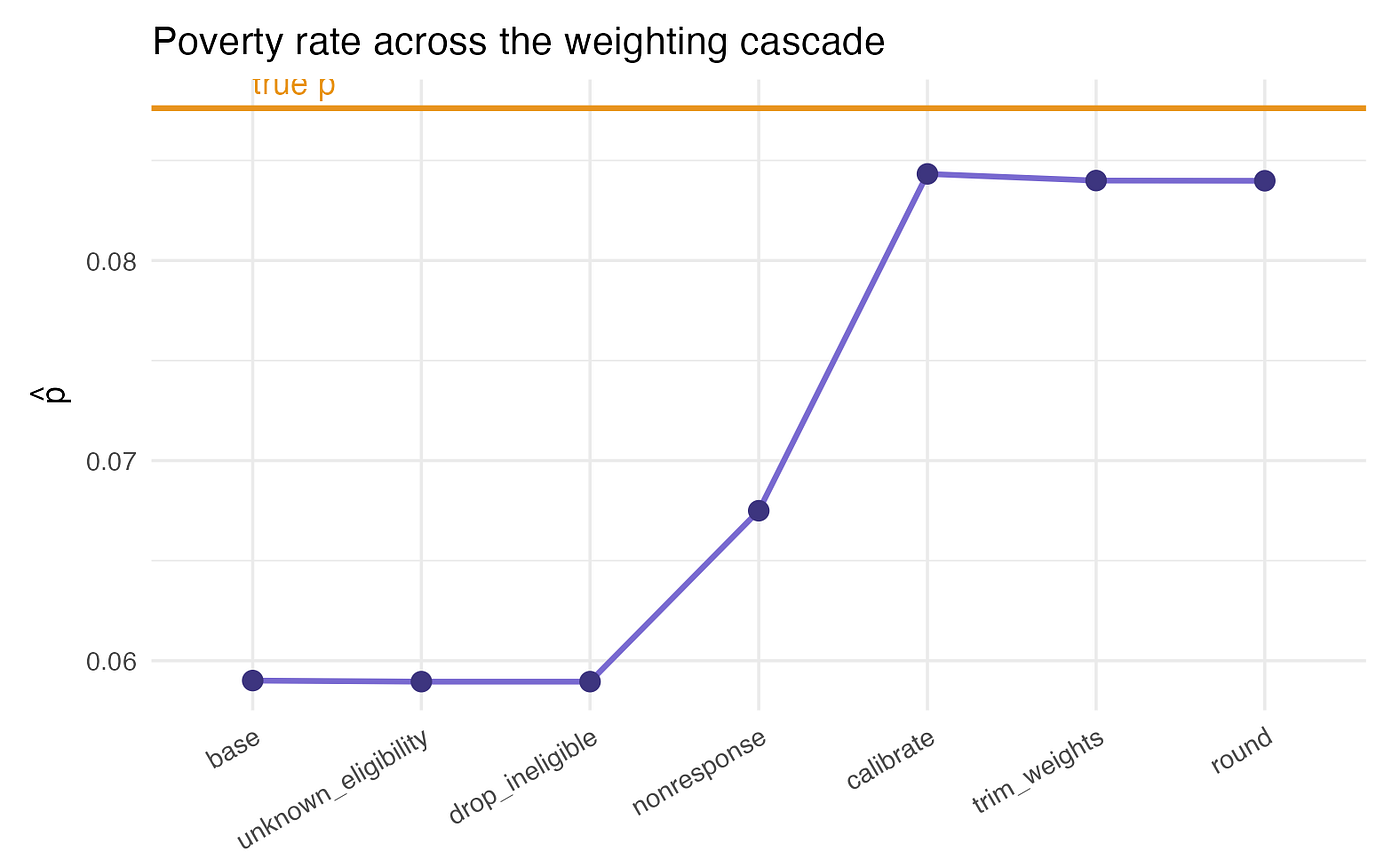
Computing the poverty rate at each stage tells the story. The naive base estimate is badly biased downward, 0.059 against the true 0.0876, because the poor responded less. The nonresponse adjustment by stratum recovers the between-strata part (0.068), and calibration to age, sex and region recovers most of the rest (0.084), landing close to the truth. A small residual gap remains, which is honest: the adjustments only use the frame and the calibration margins, not the outcome itself.

The Kish design effect climbs from 1.08 at base to 1.42 after calibration, the price of the unequal weighting the corrections introduce.

Honest uncertainty, not just a point

A point estimate close to the truth is not enough; we need a confidence interval that reflects the design and the fact that the weighting itself was estimated. weightflow’s bootstrap re-samples primary sampling units within strata and re-applies the entire recipe on each replicate:

boot <- bootstrap_weights(fitted, replicates = 1000,
                         strata = "strata", psu = "psu")
boot_mean(boot, "poverty")     # estimate, SE and 95% CI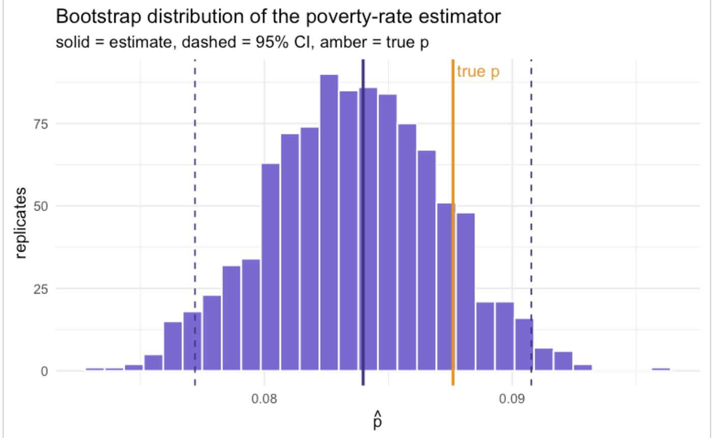

The resulting 95% interval covers the true poverty rate. So the pipeline does not just get close by luck; it recovers the parameter with uncertainty you can defend. Because the replicate weights carry both the sampling design and the weighting cascade, you can also hand them to survey/srvyr via as_svrepdesign() and analyse any estimator or domain as usual.

Is it fast enough to re-run everything?

Re-running the whole recipe on every replicate sounds expensive, so here are real numbers. On a laptop (Apple M4), preparing the full recipe on ~79,000 records takes under half a second, the point estimate and all its diagnostics are essentially instant. The 1,000-replicate bootstrap, which re-estimates the entire pipeline a thousand times, takes about six minutes. Full design-based inference on real survey data, on a single machine.

Takeaways

Two things I want survey practitioners to take from this. First, weighting is a sequence of decisions, and writing it as one explicit recipe makes it reproducible, auditable and easy to hand over, the recipe is the institutional asset, not just the final weights. Second, if any of those decisions were estimated from the data (nonresponse models, calibration), your variance should say so; re-running the recipe per replicate is how you get standard errors that tell the truth.

Everything here is reproducible from the public ECH file plus seeded code. The full walkthrough, with all the figures, is in the package’s ECH case-study article.

• Docs and the full ECH case study: https://jpferreira33.github.io/weightflow/
• CRAN: https://CRAN.R-project.org/package=weightflow
• Source: https://github.com/jpferreira33/weightflow

Cross-posted to R-bloggers.