Accelerating the Grid: Enhanced Solving of Optimal Power Flow with Graph Neural Networks

By Yassine Guennoun, Edouard Rabasse and Hippolyte Wallaert, as part of the Stanford CS224W course project

Energy is the backbone of our economy, and electricity has become central to fulfilling the ambitions of the AI revolution. At the heart of these energy considerations lies the field of grid optimization, which computes the optimal power distribution over available generators to fulfill consumer demand.

Solving this problem effectively is crucial for maximizing the efficiency and stability of the energy distribution system. However, current industry standards rely on iterative numerical solvers; while these solve the problem exactly, they come at the cost of significant computational overhead and time complexity.

Solving this problem faster is no longer just a luxury, it is a necessity. As grid operators need to adapt grid configurations in real-time to meet fluctuating demands, the latency of traditional solvers becomes a bottleneck. A promising solution lies in Graph Neural Networks (GNNs), which can approximate solutions almost instantly at the cost of a single inference. Whether the GNN output is used directly or fed into a traditional solver as a “warm start,” this acceleration framework is essential for scaling Optimal Power Flow (OPF) to meet the challenges of the modern grid.

Understanding Optimal Power Flow

Grid optimization setup

To apply machine learning to energy distribution, we must first map the physical reality of an electrical grid to a mathematical structure we can compute: a graph.

In a physical power grid, electricity is generated at power plants, transmitted across vast distances via high-voltage lines, and delivered to cities and factories. In graph theory terms, we represent this network as a graph G=(V,E).

• Nodes (V): Represent “buses” which are the junction points in the grid (e.g., power stations, substations, or consumption hubs).
• Edges (E): Represent the transmission lines connecting these buses.

This mapping allows us to treat the grid state as a set of features residing on these nodes and edges.

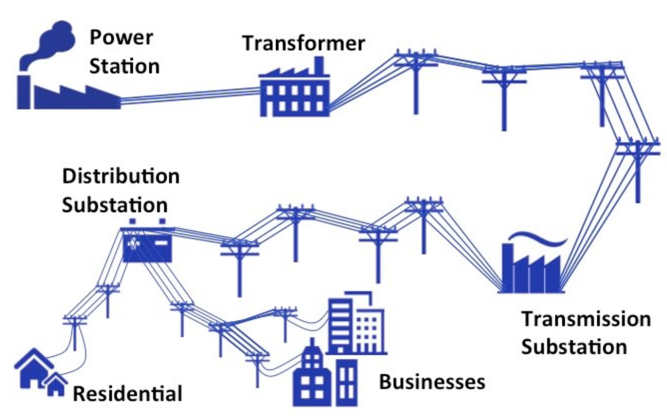
Figure 1: From infrastructure to information: Mapping physical power grid components (left) to their graph representations (right)

Crucially, not all nodes in this graph are identical. Understanding the heterogeneity of the grid is key to defining our model inputs:

1. Generator Buses (PV Nodes): These define the supply. They are controlled by active power generation (P) and voltage magnitude (∣V∣).
2. Load Buses (PQ Nodes): These define the demand. They are characterized by their consumption of active power (P) and reactive power (Q).
3. Reference Bus (Slack Bus): A single node acts as the reference for phase angles and balances the system’s total power.

Similarly, the edges (transmission lines) possess static features determined by physics, specifically impedance and admittance, which dictate how easily current flows between nodes.

The Optimal Power Flow problem

Before we can optimize the grid, we must define the physics that govern it. In an Alternating Current (AC) grid, the flow of power is dictated by Kirchhoff’s laws. For every node i in the graph, the net power injected must equal the power flowing out to connected neighbors.

This relationship is captured by the AC Power Flow equations:

Where:

• P_i​, Q_i​ are the active and reactive power injections at node i.
• ∣V∣ is the voltage magnitude and θ is the phase angle.
• G_ik​ and B_ik​ represent the conductance and susceptance (physical properties) of the transmission lines connecting nodes i and k.

The Optimal Power Flow problem asks a harder question: given the fixed demands at Load nodes, how should we configure the Generators to minimize the total cost of operation while satisfying physical and safety constraints ?

Mathematically, this is a non-convex, constrained optimization problem. We aim to minimize a cost function subject to:

• Equality Constraints: The power flow equations above (physics must hold).
• Inequality Constraints: Voltage limits (V_min​≤∣V∣≤V_max​) and thermal limits on lines (wires shouldn’t melt).

The Machine Learning Task: Node Regression

Traditionally, solvers find the optimal ∣V∣ and θ iteratively. In our deep learning approach, we reframe this as a supervised node regression task. Given a graph where:

• Input features X represent the grid topology, line impedances, and fixed load demands (P_d​,Q_d​).
• Target labels Y are the optimal operational values computed by a classical solver.

The specific targets depend on the node type, making the task heterogeneous:

• For Load Nodes: We predict the voltage magnitude ∣V∣ and phase angle θ.
• For Generator Nodes: We predict the Active Power (P_g​) and Reactive Power (Q_g​) setpoints, alongside their voltage states.

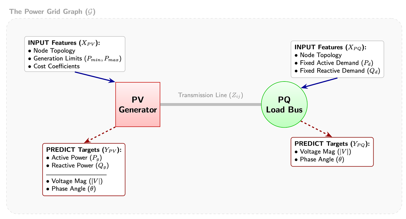
Figure 2: Power Grid Graph

Our goal is to train a Graph Neural Network f_ϕ​ such that f_ϕ​(X)≈Y, predicting the optimal grid state in a single forward pass.

Dataset & Experimental Setup

To validate our approach, we utilize the IEEE 118-bus system [1], a canonical benchmark in power systems research. This dataset represents a portion of the American Electric Power System (in the US Midwest) as of 1962 and contains 118 buses, 19 generators, and 177 transmission lines.

Figure 3: Official setup for the IEEE 118 power grid.

Generating enough data to train a deep neural network requires solving thousands of OPF scenarios. We rely on the PowerGraph dataset [2], a recently released benchmark specifically tailored for Graph Neural Networks. The authors used the physics-based MATPOWER solver to generate ground-truth labels for thousands of grid states, ensuring our model learns from highly accurate physical simulations.

Since graph datasets can be memory-intensive, efficient loading is critical. We leverage the InMemoryDataset base class from PyTorch Geometric (PyG). This allows us to load the entire processed dataset into RAM (CPU or GPU) once, drastically speeding up training epochs compared to reading from disk on the fly.

Here is the structure we used to load the data:

import torch
from torch_geometric.data import InMemoryDataset, Data

class OPFDataset(InMemoryDataset):
    def __init__(self, root, transform=None, pre_transform=None):
        super().__init__(root, transform, pre_transform)
        # Load the already processed data from disk to RAM
        self.data, self.slices = torch.load(self.processed_paths[0])

    @property
    def raw_file_names(self):
        return ['raw_grid_data.pt']

    @property
    def processed_file_names(self):
        return ['opf_data.pt']

    def process(self):
        raw_data_list = torch.load(self.raw_paths[0]) 

        data_list = []
        for case in raw_data_list:
            # Extract Node Features (P, Q, V, etc.)
            x = torch.tensor(case['x'], dtype=torch.float)

            # Extract Graph Topology & Line Physics
            edge_index = torch.tensor(case['edge_index'], dtype=torch.long)
            edge_attr = torch.tensor(case['edge_attr'], dtype=torch.float)

            # Extract Targets 
            y = torch.tensor(case['y'], dtype=torch.float)

            data = Data(x=x, edge_index=edge_index, edge_attr=edge_attr, y=y)
            data_list.append(data)

        # Collate and save
        data, slices = self.collate(data_list)
        torch.save((data, slices), self.processed_paths[0])

Heterogeneous Graphs: Towards SOTA Regression Performance

Understanding the Heterogeneous Shift

Standard Graph Neural Networks often process every node using a shared transformation, applying a uniform set of learnable weights across the entire grid. However, as established in our dataset setup, a nuclear power plant (PV node) and a residential neighborhood (PQ node) are fundamentally different entities.

Heterogeneous graphs solve this by explicitly defining multiple node and edge types [3], each handled by distinct neural networks. These models extend the concept of message passing by using type-specific functions. In our case, while the physical transmission lines might look identical, the relationship dictates the physics. A message passing from a Generator → Load carries supply-side constraints (e.g., generation limits), whereas a message flowing from Load → Load conveys demand-side dynamics (e.g., voltage couplings).

By defining three node types (PQ, PV, Slack) and assigning distinct encoding networks to each, we allow the model to learn “expert” sub-functions for each entity’s unique physics, rather than forcing a single shared weight matrix to average out these complex dynamics.

Figure 4: Heterogeneous GNN (physics-aware).

The Architecture: Heterogeneous Graph with Global Attention (HeGGA)

To capture both the local laws of physics and the grid-wide constraints, we designed a hybrid architecture that processes the graph in three distinct stages.

First, heterogeneous encoders (independent MLPs) project each node type into a shared latent space, allowing the model to immediately distinguish a Generator’s control variables from a Load’s fixed demands. In the message-passing phase, nodes exchange local messages weighted by line physics (conductance and susceptance), while a parallel global attention mechanism [4] summarizes the entire grid state into a single context vector, capturing long-range voltage dependencies that simple neighbor-passing misses. To guide this multi-head attention with structural information, nodes are enriched with Laplacian positional encodings that inject the graph’s topology directly into the latent space. This “local-plus-global” update is repeated for several layers, allowing nodes to progressively refine their understanding of the grid state before type-specific decoders map the final features back to predicted electrical quantities (P,Q,∣V∣,θ).

Figure 5: The complete architecture flow. A more detailed diagram is available here.

A PyG implementation of our architecture is given below :

def hegga_forward(data, num_layers, node_encoders, edge_encoder,
                    edge_updates, node_updates, fusions, attn, decoders):

    x, edge_index = data.x, data.edge_index
    edge_attr = data.edge_attr
    src, dst = edge_index

    # ---- 1) Type-specific node encoding ----
    node_types = _infer_node_types(x[:, 2])
    pe = data.pe # assume already computed externally
    h = torch.zeros(x.size(0), node_encoders[0][0].out_features, device=x.device)
    for t in range(3):
        h[node_types == t] = node_encoders[t](torch.cat([x[node_types == t], pe[node_types == t]], dim=-1))


   e = edge_encoder(edge_attr)

    # ---- 2) L message-passing layers ----
    for edge_upd, node_upd, fusion in zip(edge_updates, node_updates, fusions):

        # (a) Edge update: MLP([h_src, h_dst, e]) + residual
        m_edge = edge_upd(torch.cat([h[src], h[dst], e], dim=-1))
        e = e + m_edge

        # (b) Aggregate edge states into nodes (sum incoming edges)
        agg = torch.zeros_like(h)
        agg.index_add_(0, dst, e)

        # (c) Node update (local residual): h_local = h + Δh
        dh = node_upd(torch.cat([h, agg], dim=-1))
        h_local = h + dh

        # (d) Global attention: h_global = Attn(h_local)
        h_global = attn(h_local)

        # (e) Fusion (local + global)
        h = fusion(h_local + h_global)

    # ---- 3) Type-specific decoding ----
    out = torch.zeros(h.size(0), decoders[0][-1].out_features, device=h.device)
    for t in range(3):
        out[node_types == t] = decoders[t](h[node_types == t])

    return out

Performance

Figure 6: MSE performance

The Impact of Grid Size : While our model consistently outperforms the baseline, the margin of improvement depends heavily on the grid topology. On small grids like the IEEE-24, a standard 5-layer message-passing network [5] can already capture the entire graph context, resulting in smaller relative gains.

However, as grid size increases (IEEE-39, UK, IEEE-118), performance gains are primarily driven by the heterogeneous message-passing backbone, while global attention contributes only marginal refinements. Our results show that simply switching to a heterogeneous architecture with type-specific MLP encoders reduces error by several orders of magnitude compared to the baseline. This indicates that the core challenge isn’t just long-range traversal, but correctly modeling the distinct physical behaviors of generators, loads, and transmission lines.

The Road to the Best Architecture : Our final design wasn’t our first guess. We iterated through several approaches to inject global context:

• Virtual Node: We first tried adding a single super-node connected to all others. This yielded a slight improvement but introduced an information bottleneck, as all global context had to be compressed through a single node embedding
• The Dominance of the Backbone (No Attention): The configuration without any attention mechanism achieves results that are nearly identical to the attention-based variants, showing that the Heterogeneous MLP backbone is the primary factor in reducing error.
• Readout-Only Attention: Restricting global attention to the final layer yields only a marginal improvement over the “No Attention” model. This minimal difference confirms that while a global readout can provide a slight refinement to the final state estimation, it is not critical for convergence.

Redundancy of Positional Encodings: Contrary to our initial assumptions, removing Laplacian positional encodings (PE) yields the optimal performance. This suggests that the necessary structural information is already intrinsic to the heterogeneity of the graph. Consequently, adding spectral positional signals becomes redundant and acts as a source of noise.

Table 1: Results on IEEE118. Mean MSE computed over random seeds, with variability of the order of 10%.

Bridging the Gap: The Trade-off Between Speed, Accuracy, and Physics

In many machine learning applications, a “good enough” prediction is acceptable. If a recommendation engine predicts a movie you mostly like, the system is a success. In grid optimization, however, the stakes are fundamentally different.

The electrical grid is governed by strict physical laws that are unbreakable in practice. A predicted grid state might have an incredibly low regression error (meaning it looks very close to the optimal solution mathematically), but if it violates the conservation of power at a single bus, it is physically impossible to implement.

The Feasibility-Optimality Dilemma

Standard GNNs are typically trained to minimize Mean Squared Error (MSE) against a ground truth. They act as curve fitters, blindly chasing the numerical targets without understanding the underlying physics.

This often leads to a dangerous disconnect:

• Pure Regression Performance: Focuses on minimizing the distance to the optimal solution (∣V∣≈V_target​).
• Physical Feasibility: Focuses on ensuring the system actually works (Power In = Power Out).

We observed that a model can achieve state-of-the-art regression scores while producing solutions that are physically invalid . For a neural solver to be useful in the real world, being “physically feasible” is just as important as being “optimal.” We need to push the boundary where these two objectives meet.

Enhancing Physical Feasibility Using the Physical Loss Component

Projecting the GNN’s output back onto the physically feasible manifold requires running an expensive iterative solver inside the training loop, effectively negating the GNN’s speed advantage. Similarly, forcing hard constraints during training often disrupts gradient flow, leading to unstable convergence.

Instead, we guide the model towards feasibility by integrating physics directly into the training objective via a Physical Loss (L_phy) term. This acts as a soft constraint, penalizing the model whenever its predicted voltage and phase states imply power flows that violate Kirchhoff’s conservation laws at any node.

We define this loss as the mean absolute error between the power injected/consumed at a node (predicted by the model or fixed by demand) and the actual power flowing into that node from its neighbors (calculated using the AC Power Flow equations based on predicted V and θ).

Mathematical formulation of the Physical Loss term

Implementing this requires differentiable operations to calculate power flow across the graph structure:

def physics_loss(pred, edge_index, edge_attr, maxs_y):
    """
    Calculates the power mismatch based on Kirchhoff's laws (AC Power Flow).

    Args:
        pred: Model predictions [N, 4] -> [Pg, Qg, V, Theta] (Normalized)
        edge_index: Graph topology [2, E]
        edge_attr: Edge attributes [E, 2] -> [Conductance G, Susceptance B] (Unnormalized!)
        maxs_y: Normalization factors for Y [1, 4]

    Returns:
        Scalar Tensor representing the average physical error (MSE of the mismatch).
    """
    # 1. Denormalization
    P_pred = pred[:, 0] * maxs_y[0]
    Q_pred = pred[:, 1] * maxs_y[1]
    V_pred = pred[:, 2] * maxs_y[2]
    theta_pred = pred[:, 3] * maxs_y[3]

    src, dst = edge_index
    G = edge_attr[:, 0]
    B = edge_attr[:, 1]

    # --- CALCULATION OF BRANCH FLOWS ---

    # Pre-calculations
    delta_theta = theta_pred[src] - theta_pred[dst]
    cos_t = torch.cos(delta_theta)
    sin_t = torch.sin(delta_theta)

    # Quadratic term (V_i^2) for the source node
    # Represents the power related to the voltage at the node itself
    vv_self = V_pred[src] ** 2 

    # Cross term (V_i * V_j)
    vv_cross = V_pred[src] * V_pred[dst]

    # Full Branch Flow Equations
    # P_ij = G * V_i^2 - V_i*V_j * (G*cos + B*sin)
    p_flow = (G * vv_self) - vv_cross * (G * cos_t + B * sin_t)

    # Q_ij = -B * V_i^2 - V_i*V_j * (G*sin - B*cos)
    # (Note: The sign of B depends on the dataset convention; B is often negative for inductive lines)
    q_flow = (-B * vv_self) - vv_cross * (G * sin_t - B * cos_t)

    # ------------------------------

    # 5. Aggregation (Sum of outgoing flows)
    # Aggregates flows from edges back to source nodes
    P_out_lines = scatter_add(p_flow, src, dim=0, dim_size=pred.size(0))
    Q_out_lines = scatter_add(q_flow, src, dim=0, dim_size=pred.size(0))

    # 6. Mismatch: Injection - Outflow = 0
    # P_pred is the NET injection (Generation - Load). 
    # Therefore, P_pred must equal P_out_lines (power flowing into the grid).
    diff_P = P_pred - P_out_lines
    diff_Q = Q_pred - Q_out_lines

    # Calculate Mean Squared Error of the physical violation
    loss_phy = torch.mean(diff_P**2 + diff_Q**2)
    return loss_phy

Balancing the Trade-off

We control the balance between fitting the ground truth and respecting physics by introducing a regularization hyperparameter, λ, into the total loss function:

By sweeping across different values of λ during training, we generate a Pareto frontier that visually quantifies this trade-off.

Figure 7: The Pareto Frontier. Every point is a training for a specific value of λ, averaged on 5 different seeds.

This plot highlights two regimes:

1. The Data-Driven Regime (Low λ) For small values of λ (the bottom-right of the curve), the model acts as a pure regressor. We observe exceptional regression accuracy (low MSE) but a persistently high physics error.

At first glance, it seems paradoxical that a model matching the ground-truth labels so closely would produce a high physical violation. However, this discrepancy reveals a limitation in the dataset rather than the model. In reality, the strict nodal balance equation used to generate the ground truth includes the effects of Shunt Conductances (g and b), as shown in Equation (4):

Our simplified physics loss omits the g and b terms because these values are not observed in the input features or predicted by the model. Consequently, the “error” observed in this regime is actually the physical magnitude of the unmodeled shunt power. The model fits the data perfectly but wont give a loss equal to 0 because of this remaining term.

2. The Physics-Forced Regime (High λ) In the top-left region of the plot, we see points corresponding to high values of λ (10−2 and above). Here, the penalty for physics violation becomes dominant. To minimize the physics loss the model focuses more on satisfying the equation P_in​ = P_out​ than on accurate prediction. The result is a lower physics error but a drastically higher regression error (MSE). The model is approaching a grid state that satisfies our simplified laws but deviates significantly from the true optimal state.

We initially hypothesized that the physical loss term (L_phy​) would act as a strong inductive bias, accelerating convergence by restricting the search space to valid grid states. However, our experiments reveal a more nuanced interaction the regularization term either has no influence (if too small) on the convergence, or guides the model toward wrong predictions (if too big). This suggests that the simplified physical laws we enforce act as a rigid approximation of the complex, high-fidelity simulations used to generate the dataset. Therefore, treating the physics loss as a hard constraint forces the model to prioritize an idealized mathematical consistency over the empirical reality of the optimal grid states, leading to a degradation in predictive accuracy when the physics weight (λ) is too large.

Conclusion

As seen in Figure 7, our model HeGGA establishes a new standard by outperforming the baseline significantly in terms of both prediction accuracy and physical feasibility. This simultaneous improvement highlights that by explicitly modeling the grid’s heterogeneity and injecting global context via attention, the network can learn the complex interplay of voltage and power more effectively than standard message-passing approaches.

Our experiments with the Pareto frontier reveal a critical insight for future research: while physics-informed loss functions are theoretically appealing, they are limited by the fidelity of the mathematical equations used during training. When the loss function simplifies reality (e.g., ignoring shunt conductances), forcing the model to strictly obey it can actually degrade performance against high-fidelity ground truth data [6, 7].

Ultimately, the most immediate value of this accelerated solver lies not in replacing classical methods entirely, but in augmenting them. Even with a small degree of physical error, the GNN’s predictions are incredibly close to the optimal state.

• Stand-alone Inference: Useful for rapid contingency analysis where approximate speed is more critical than 100% precision [8].
• Warm Start: The GNN output can serve as the initial guess for a Newton-Raphson solver. Instead of starting from a “flat start,” the solver begins near the solution, potentially reducing convergence time from seconds to milliseconds.

By combining the fast inference of Graph Neural Networks with the rigorous guarantees of classical control theory, we pave the way for a smarter, more responsive power grid.

References

[1] A. R. Al-Roomi, “Power Flow Test Systems Repository,” Dalhousie University, Electrical and Computer Engineering, Halifax, Nova Scotia, Canada, 2015. [Online]. Available: https://al-roomi.org/power-flow

[2] A. Varbella, K. Amara, B. Gjorgiev, M. El-Assady, and G. Sansavini, “PowerGraph: A power grid benchmark dataset for graph neural networks,” arXiv preprint arXiv:2402.02827, 2024.

[3] M. Schlichtkrull, T. N. Kipf, P. Bloem, R. van den Berg, I. Titov, and M. Welling, “Modeling Relational Data with Graph Convolutional Networks,” in European Semantic Web Conference (ESWC), 2018.

[4] P. Veličković, G. Cucurull, A. Casanova, A. Romero, P. Liò, and Y. Bengio, “Graph Attention Networks,” in International Conference on Learning Representations (ICLR), 2018.

[5] V. P. Dwivedi, C. K. Joshi, T. Laurent, Y. Bengio, and X. Bresson, “Benchmarking Graph Neural Networks,” Journal of Machine Learning Research (JMLR), vol. 24, no. 43, pp. 1–48, 2023.

[6] V. Eeckhout, H. Fani, M. U. Hashmi, and G. Deconinck, “Improved Physics-Informed Neural Network based AC Power Flow for Distribution Networks,” arXiv preprint arXiv:2409.09466, 2024.

[7] O. Arowolo and J. L. Cremer, “Towards Generalization of Graph Neural Networks for AC Optimal Power Flow,” arXiv preprint arXiv:2510.06860, 2025.

[8] A. S. A. Awad et al., “Web application for power grid fault management,” in 2016 6th International Conference on Intelligent and Advanced Systems (ICIAS), 2016.

Hardware & Computational Resources

To ensure consistent benchmarking across our experiments, all models were trained on workstations adhering to a standardized hardware specification. This setup provided sufficient VRAM to leverage PyTorch Geometric’s InMemoryDataset, allowing us to load the entire processed IEEE-118 PowerGraph dataset directly into GPU memory.

Workstation Specifications:

• GPU: NVIDIA RTX A5000
• VRAM: 24 GB GDDR6
• CUDA Environment: Version 13.0
• Driver Version: 580.105.08

Code

Find our implementation here: https://github.com/h1ppox99/powerflow-gnn