Machine Learning Series (Part 25) — Too Fast or Too Slow? The Role of Learning Rate in Gradient Descent

Dear readers, we are in the arc of knowing about the gradient descent which is the engine that optimizes the ML models. From part 22 to 24 we had seen various measures of errors — MAE, MSE, RMSE etc , the cost function and the need of optimization and finally we saw about the calculation of the gradient of a curved surface in the last part. Today we shall see how models make use of the calculated gradient to find the most minimum point in the loss surface. The key role that is behind reaching the lowest point in order to bring the loss value close to 0 is ‘learning rate’. We shall discuss it more clearly today. Also, the answer to the question of why don’t we choose Mean Absolute Error (MAE) over Root Mean Squared Error (RMSE) will be seen today.

In part 24, we learnt what slope is and how the slope is calculated for a linear function and non linear (curved) function. For a curved surface which is in the form of y = x² , the slope is calculated via the ‘derivative’, also we deep dived into how the derivative is found by taking an infinitesimally small value close to the point in the curve. Using this, We shall find out the derivative of our loss function MSE. Mostly the gradient descent process is applied to MSE as reducing Mean Squared Error automatically reduces Root Mean Squared Error. Another reason, applying the derivatives to MSE is simpler while RMSE is complex.

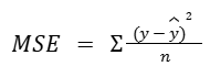
We know that

Now if we differentiate the MSE function, that is if we would like to like to find the gradient of it, then it becomes:

We know that

The predicted value is found by y = mx+c. For every observation i, it is denoted as

Now if have this substituted in the MSE, then its gradient becomes,

With this the gradient doesn’t stop, we have only differentiated the entire loss function using our rule

Now, by the concept of chain rule, we should also differentiate the y hat which is the function of the slope. Doing so, differentiating

with respect to m becomes

c is constant, for a constant slope is 0 hence it vanishes.

Applying this overall, the gradient of MSE is

We can place the minus in the front, the final formula looks like:

Now using this gradient, we will get to know the direction by which we have to move to the lowest point. Our loss function will be like a widespread sheet. If we consider just a single attribute that is y being a target variable is dependent on just a single attribute x, then our loss function might look like below:

In the above picture, Maxima refers to peak points in a curve. The highest peak in the entire curve is called the global maximum, while other peaks that are higher than their nearby points are called local maxima. Similarly, minima refers to the low points in a curve. The lowest point in the entire curve is called the global minimum, while other low points that are lower than their nearby points are called local minima.

Note: “Maximum” and “minimum” refer to a single point (singular), while “maxima” and “minima” are their plural forms. For example, one highest point is called a global maximum, whereas multiple peak points are called local maxima. Similarly, one lowest point is a global minimum, and multiple low points are called local minima.

Our goal is to reach the global minimum which is the lowest point in the loss function. If there are two dependent variables, the loss function would be represented in 3D as shown below.

Note: Here, both the slope (m) and intercept c are parameters of the model, and the loss depends on both, which is why we can visualize it as a 3D surface. While differentiating with respect to one parameter (for example, m), the intercept c is treated as a constant and its derivative becomes 0. However, in the overall loss function, c is still a parameter that also gets updated during training.

If there are more dimensions, then it is difficult to visualize as we can only view upto 3D. But the purpose to reach the global minimum would be accomplished by the process of the gradient descent no matter the number of dimensions (though it is 2D or 3D or more) .

For simplicity, In the below sections, I demonstrated gradient descent using only one parameter (the slope). In practice, models usually have multiple parameters (like slope and intercept), and gradient descent updates each of them separately using their respective gradients.

So far, we got to know the direction to be moved after finding out the gradient. Now, how do we move to the point is the question. We update this slope (which is the parameter in this case) using:

Since we are working with a single variable, this parameter is the slope of the line. So intuitively, we are updating the slope using the gradient.

In the above equation, there is a new term — learning rate, let’s see about it. Imagine, you are at a hill, gone for a trek and you are supposed to reach the lowest point of the hill post climbing the summit. Assume that the slope of the surface at the current position is +4. As we had seen already, we move in the direction opposite to the slope because the slope +4 indicates that the surface is increasing, so moving in the same direction of the slope leads to a further high steep position. Thus we move opposite to it. Now, moving opposite is fine. But at what steps do we move? Do we take big steps or tiny steps? Here is where today’s hero ‘learning rate’ enters into the scene. The learning rate determines how big our step should be. The same scenario is applied in gradient descent as well, how big the step of the model should be.

Let’s see through an example.

If the current parameter value is 10 and the calculated gradient is +4, then the new parameter for a learning rate of 0.1 will be:

New Parameter = Old Parameter — (learning rate x gradient)

New Parameter = 10 — (0.1 x 4)

New Parameter = 9.6

Here is a simple analogy to understand the weight (parameter), gradient and the learning rate:

• m (parameter) = your position on the map
• gradient = slope of the terrain under your feet
• learning rate = step size

Now you might ask a question, taking big steps is only correct because it leads us to the lowest point (global minimum) so quickly. While that is true, now imagine the trek is happening in a blindfolded way and somehow you have reached closer to the lowest point but not exactly reached. Then at this point, taking a big step might take you beyond the global minimum, that is to the next higher/increasing point rather than the lowest point. The same is applied to the ML model as well. You can think of the ML model too as a blindfolded person. It cannot see where exactly the lowest point is, only based on the learning rate and the new updated parameter value, it can reach the global minimum point.

It’s time to recollect the MAE and MSE that we saw in our part 22. We ended our blog with a question of what does the difference between 3.5 and 3.53 make? The answer is, MSE is easier for the model to converge meaning that it helps to take steps that can reach the global minimum, on the other hand for MAE, the gradient of the error function is always a constant magnitude. So taking steps using MAE might result in the model to jump back and forth on the surface and can cause oscillations near the minimum and slow convergence. You can recollect the plot of the errors in part 23 where the plot of MAE was V shaped while the plot of MSE was a parabola. Here is the actual reason why MAE oscillates:

The loss function of MAE is represented as

When we substitute for y hat, it becomes

When we differentiate MAE with respect to m, the gradient becomes either +x or -x

This depends on whether the predicted value is greater than or less than the actual value.

If the predicted value mx+c is less than the actual value, the gradient becomes -x

Here is an example to support:

Assume x = 2, y = 5 , learning rate = 0.1, m=1

predicted y (y hat) = 1 x 2 = 2

Error = actual-predicted = 5–2 = 3

gradient of MAE with respect to m gives -x

substituting the value in the gradient gives -2. Based on this calculated gradient, we update the parameter.

If the predicted value is greater than the actual value, the gradient becomes +x. You can try out an example by yourself as like the above case.

Since the gradient does not gradually reduce near the minimum and keeps switching between +x​ and ​ -x, the model can overshoot and oscillate around the minimum.

Coming back to the learning rate, the balance between the big steps and the tiny steps is generally an experiment. Trying out different values of learning rate like 0.1,0.01,0.001,0.0001 produces various error values. Based on the error values, we can fix which learning rate was the best for the most optimized results of the ML model.

In the next blog, we shall see about the different types of gradient descent algorithm — stochastic gradient descent, batch gradient descent, mini batch gradient descent.