Single-Qubit Gates: X, Y, Z, Hadamard — A Visual Tour

Visualising Quantum Gates on the Bloch Sphere

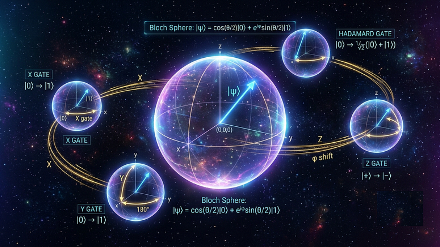
Quantum computing introduces a fascinating paradigm in which information exists in superposition. Single-qubit gates are the fundamental building blocks of quantum circuits, rotating and manipulating qubit states on the Bloch sphere. In this article, we’ll visualise how the X, Y, Z, and Hadamard gates transform a qubit’s state vector on the Bloch sphere, making these abstract mathematical operations tangible and intuitive.

We’ll use Qiskit with the Aer simulator to create visual representations of these gates. The code is designed to run in Jupyter Notebook or Google Colab, making it accessible for both beginners and experienced developers exploring quantum computing.

Setting Up Your Environment

First, let’s set up our Python environment. I recommend using a virtual environment for clean dependency management:

For Windows:

python -m venv medium_quantum_venv
medium_quantum_venv\Scripts\activate

For macOS/Linux:

python3 -m venv medium_quantum_venv
source medium_quantum_venv/bin/activate

Now install the required packages:

pip install qiskit qiskit-aer matplotlib numpy

For the complete notebook with all visualisations, check out the GitHub repository.

Importing Required Libraries

Create a new Jupyter notebook and start with these imports:

from qiskit import QuantumCircuit, transpile
from qiskit_aer import AerSimulator
from qiskit.visualization import plot_bloch_multivector
import matplotlib.pyplot as plt
import numpy as np
from IPython.display import display

Helper Function for Visualisation

We’ll create a reusable function to visualise any quantum circuit’s state on the Bloch sphere:

def visualize_state(circuit, title="State Vector"):
    # Visualize the quantum state on the Bloch sphere
    simulator = AerSimulator()
    circuit.save_statevector()
    result = simulator.run(circuit).result()
    statevector = result.get_statevector(circuit)

    fig = plot_bloch_multivector(statevector)
    fig.suptitle(title, fontsize=12)
    plt.show()
    return statevector

The Identity Gate (Baseline)

Let’s start with the identity gate to see our initial state:

# Create a circuit with a single qubit
qc = QuantumCircuit(1)

# # Visualize the initial state (|0⟩)
state = visualize_state(qc, "Initial State: |0⟩")
print(f"State vector: {state}")

# plot_bloch_multivector returns a Figure object
fig = plot_bloch_multivector(state, title="Identity Gate (|0⟩)")

# Use display() to force Jupyter to render the figure in a loop
display(fig)

Expected Output:

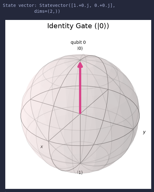
• A Bloch sphere showing the state vector pointing to the north pole (|0⟩)
• State vector printed: [1.+0.j 0.+0.j]

The Bloch sphere is a 3D sphere, with the state vector (blue arrow) pointing to the top (representing |0⟩).

X Gate (NOT Gate)

The X gate flips the qubit state, mapping |0⟩ to |1⟩ and vice versa:

# Create circuit and apply X gate
qc_x = QuantumCircuit(1)
qc_x.x(0)  # Apply X gate

# Visualize the result
state_x = visualize_state(qc_x, "X Gate Applied")
print(f"State vector after X: {state_x}")

# plot_bloch_multivector returns a Figure object
fig = plot_bloch_multivector(state_x, title="X Gate (|1⟩)")

# Use display() to force Jupyter to render the figure in a loop
display(fig)

Expected Output:

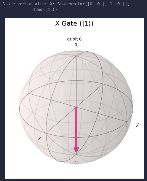
• Bloch sphere showing the state vector pointing to the south pole (|1⟩)
• State vector printed: [0.+0.j 1.+0.j]

The X gate rotates the state vector by 180° around the X-axis, moving it from the north pole to the south pole of the Bloch sphere.

Y Gate

The Y gate applies a 180° rotation around the Y-axis with a phase factor:

# Create circuit and apply Y gate
qc_y = QuantumCircuit(1)
qc_y.y(0)  # Apply Y gate

# Visualize the result
state_y = visualize_state(qc_y, "Y Gate Applied")
print(f"State vector after Y: {state_y}")

# plot_bloch_multivector returns a Figure object
fig = plot_bloch_multivector(state_y, title="Y Gate (|i⟩)")

# Use display() to force Jupyter to render the figure in a loop
display(fig)

Expected Output:

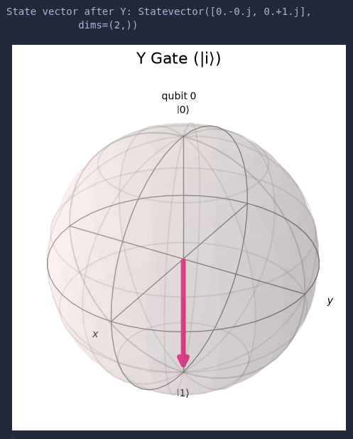
• Bloch sphere showing the state vector pointing to the south pole (|1⟩) with a phase
• State vector printed: [0.-0.j 0.+1.j]

The Y gate rotates the state vector 180° around the Y-axis, reaching the south pole with a π/2 phase shift.

Z Gate (Phase Flip)

The Z gate introduces a phase flip without changing the basis state:

# Create circuit and apply Z gate
qc_z = QuantumCircuit(1)
qc_z.z(0)  # Apply Z gate

# Visualize the result
state_z = visualize_state(qc_z, "Z Gate Applied")
print(f"State vector after Z: {state_z}")

# plot_bloch_multivector returns a Figure object
fig = plot_bloch_multivector(state_z, title="Z Gate (|0⟩)")

# Use display() to force Jupyter to render the figure in a loop
display(fig)

Expected Output:

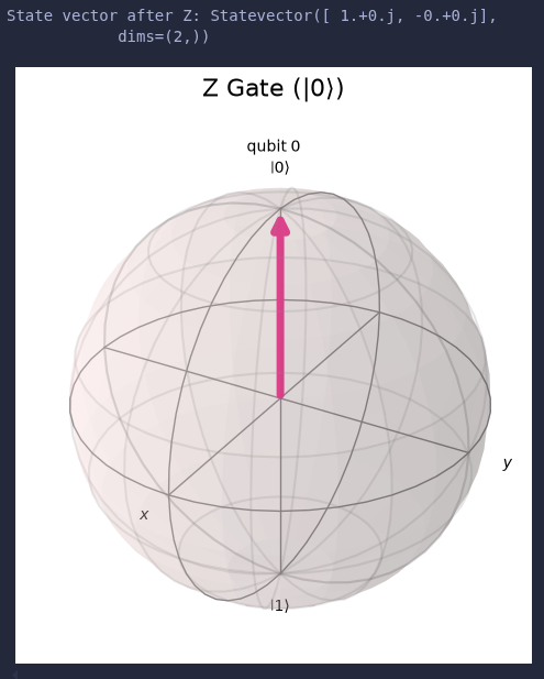
• Bloch sphere showing the state vector at the north pole (|0⟩) with a phase
• State vector printed: [ 1.+0.j -0.+0.j]

The Z gate leaves the |0⟩ state unchanged (since it’s in the north pole) but would flip the phase of |1⟩. The Bloch sphere visualisation shows the vector at the same position (north pole), but note the phase difference in the state vector.

Hadamard Gate (Superposition Creator)

The Hadamard gate creates equal superposition states:

# Create circuit and apply Hadamard gate
qc_h = QuantumCircuit(1)
qc_h.h(0)  # Apply Hadamard gate

# Visualize the result
state_h = visualize_state(qc_h, "Hadamard Gate Applied")
print(f"State vector after Hadamard: {state_h}")

# plot_bloch_multivector returns a Figure object
fig = plot_bloch_multivector(state_h, title="Hadamard Gate (|+⟩)")

# Use display() to force Jupyter to render the figure in a loop
display(fig)

Expected Output:

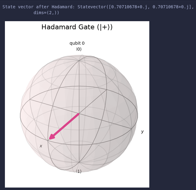
• Bloch sphere showing the state vector pointing along the X-axis (equator)
• State vector printed: [0.70710678+0.j 0.70710678+0.j]

The Hadamard gate creates a superposition state (|0⟩ + |1⟩)/√2, which is visualised as a state vector pointing to the equator of the Bloch sphere.

Visualising All Gates Together

Let’s display all gate effects in one figure for comparison:

# Define base circuits
gates = [
    ("Identity (|0⟩)", QuantumCircuit(1)),
    ("X Gate (|1⟩)", QuantumCircuit(1)),
    ("Y Gate (|i⟩)", QuantumCircuit(1)),
    ("Z Gate (|0⟩)", QuantumCircuit(1)),
    ("Hadamard Gate (|+⟩)", QuantumCircuit(1)),
]

# Apply operations
gates[1][1].x(0)
gates[2][1].y(0)
gates[3][1].z(0)
gates[4][1].h(0)

# Initialize simulator
simulator = AerSimulator()

# Simulate and display each Bloch sphere
for label, circuit in gates:
    circ_copy = circuit.copy()
    circ_copy.save_statevector()

    result = simulator.run(circ_copy).result()
    statevector = result.get_statevector(circ_copy)

    # plot_bloch_multivector returns a Figure object
    fig = plot_bloch_multivector(statevector, title=label)

    # Use display() to force Jupyter to render the figure in a loop
    display(fig)

Expected Output:

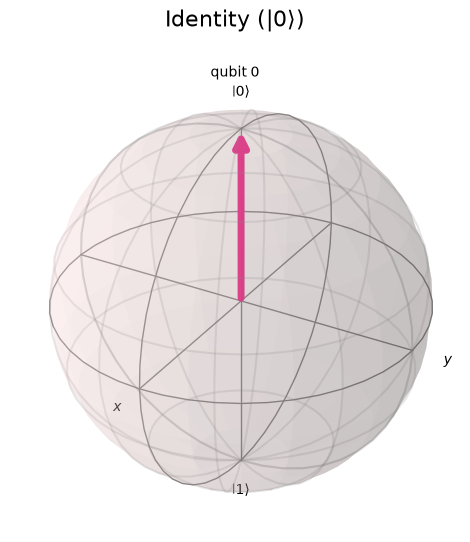
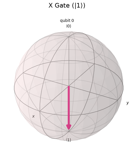
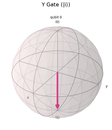
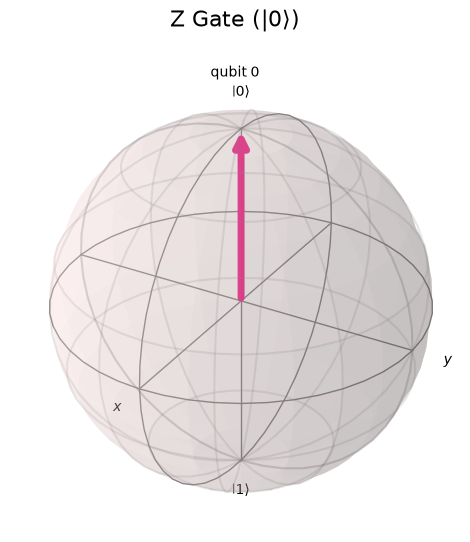
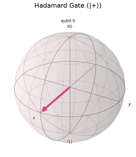
A series of Bloch spheres showing each state individually:

• Identity: Vector at north pole (|0⟩)
• X: Vector at south pole (|1⟩)
• Y: Vector at the south pole with phase (i|1⟩)
• Z: Vector at north pole (|0⟩ with phase)
• Hadamard: Vector on equator (|+⟩ superposition)

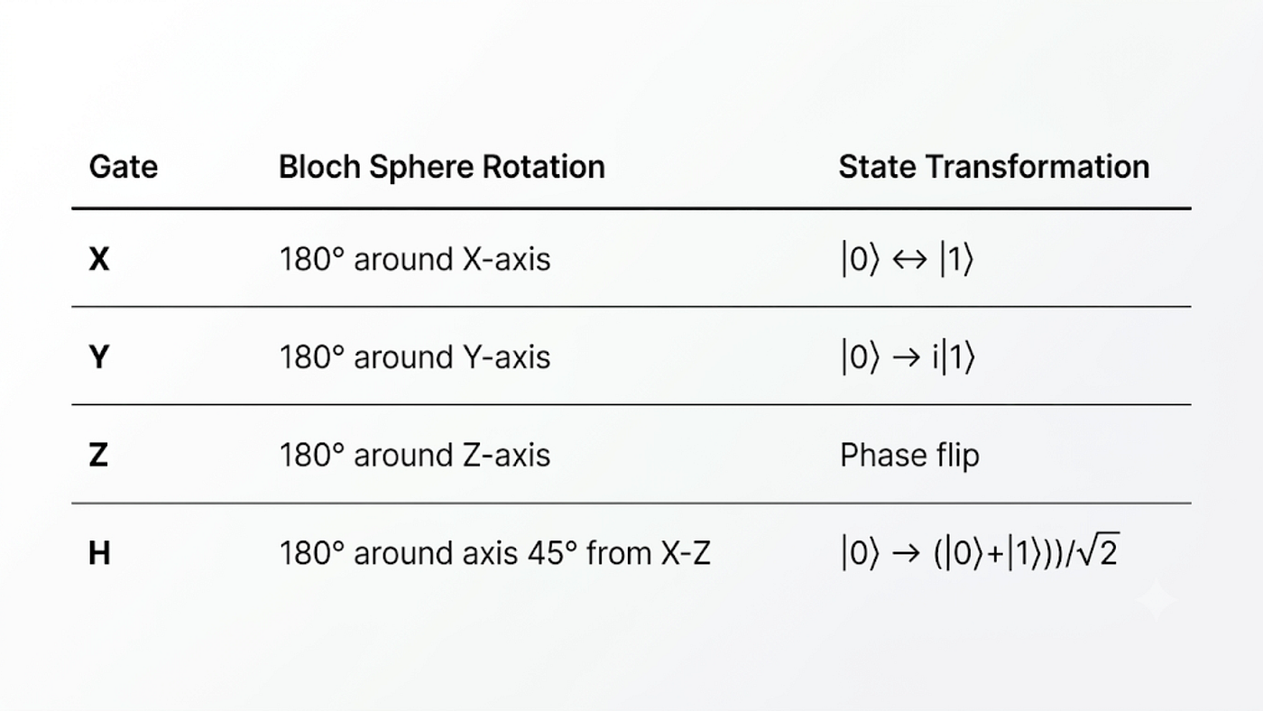
Summary of Gate Operations

Conclusion

Visualising quantum gates on the Bloch sphere provides an intuitive understanding of how these fundamental operations transform qubit states. The X, Y, Z, and Hadamard gates represent different rotations in the quantum state space:

• X and Y gates change the basis state (|0⟩ to |1⟩), but with different phase characteristics
• The Z gate introduces phase shifts without changing the basis
• The Hadamard gate creates a superposition, a uniquely quantum feature with no classical analogue

These gates form the foundation of quantum algorithms, and understanding their geometric interpretation on the Bloch sphere is crucial for developing quantum intuition. The visual approach we’ve taken here makes these abstract concepts accessible and memorable.

The complete code is available in the GitHub repository linked above. Feel free to experiment by modifying the initial state or applying sequences of gates to see how the state vector moves across the Bloch sphere!