2D Heat Conduction: PINN vs Finite Difference Method

A Practical Comparison on a Classical Benchmark Problem

Abstract

Like in all other areas, deep learning has been mostly utilized in recent engineering applications and one of them is physics-informed neural network (PINN). PINN is highly new in the area of providing solutions to the engineering problems by being able to utilize the fundamental physics of engineering systems. Innovation provided through PINNs is direct usage of partial differential equations of various engineering problems in loss function. This ability separates PINNs from other neural network applications in the area of providing solutions to the engineering problems based on a physical reality. In this study, well-known 2D Heat Conduction equation on square shape domain will be solved with both Finite Difference Method and PINN. It has been showed that PINNs can perform as accurate as Finite Difference Method based on solving of the 2D Heat Conduction equations.

1. Introduction

The heat conduction (diffusion) equation is a fundamental partial differential equation (PDE) in physics and engineering. It governs a wide range of phenomena, including thermal diffusion, mass transport, chemical diffusion, and even probability propagation in stochastic processes.

Traditionally, such equations are solved using grid-based numerical methods, among which the Finite Difference Method (FDM) is one of the most widely used. FDM discretizes both space and time and advances the solution in a physically intuitive, step-by-step manner. Its simplicity, stability properties, and predictability make it a standard tool in scientific computing.

More recently, Physics-Informed Neural Networks (PINNs) have been introduced as an alternative paradigm for solving PDEs. Rather than discretizing the governing equations explicitly, PINNs approximate the solution with a neural network and enforce the governing physics through the loss function by minimizing the PDE residual. From this information, it can be pointed out that PINNs limits the classic data-driven neural networks through reality of physics.

In a typical PINN, through automatic differentiation, partial derivatives of the neural network have been computed, and, in this way, it is allowed that PDEs back propagate through the layers of neural networks. This physics-informed view, transitioning from governing equations to learning through weight updates, allows neural networks to achieve improved generalization on real-world problems.

While PINNs have shown promise — especially in inverse problems and data-driven settings — their performance on classical forward benchmark problems must be carefully evaluated.

In this project, we perform a direct and controlled comparison between:

• a classical Finite Difference Method (FDM) solver, and
• a Physics-Informed Neural Network (PINN)

for a well-defined 2D transient heat conduction problem with a known analytical solution. The comparison focuses on accuracy, stability, and physical behavior over time.

2. Problem Definition

Consider a 2D transient heat equation on a unit square domain:

Homogeneous Dirichlet boundary conditions on all boundaries:

The initial temperature distribution is prescribed as:

For this setup, the exact analytical solution is known:

The availability of an exact solution makes this problem an ideal benchmark, allowing a clean and unambiguous evaluation of numerical accuracy.

3. Computational Setup and Reproducibility

For reproducible numerical experiments, deterministic random number generation and device-aware computation are essential, especially when training neural networks.

Implementation

device = torch.device("cuda" if torch.cuda.is_available() else "cpu")
torch.manual_seed(0)
np.random.seed(0)

This section of the code automatically selects a GPU if available, otherwise defaults to CPU execution. Fixed random seeds ensure consistent sampling of collocation points and identical neural network initialization across runs.

4. Usage of an Analytical Solution as a Reference Benchmark

The analytical solution for the 2D heat equation with homogeneous Dirichlet boundary conditions and sine initial data is derived via separation of variables and can be seen below:

Detailed derivation of this solution can be found in Strauss (Partial Differential Equations: An Introduction) [1].

This exact solution is used exclusively for post-training validation and is not used during PINN training.

Implementation

def exact_solution(x, y, t):
    return torch.exp(-2*np.pi**2*t) * torch.sin(np.pi*x) * torch.sin(np.pi*y)

5. Theory Behind the Finite Difference Method (FDM)

When the temperature gradients inside a medium are not negligible, finite difference discretization method can be used to determine the temperature distribution inside the body. With this method, the differentials of the dependent variables appearing in partial differential equations are expressed as approximate expressions and in this way, computers are used to obtain a solution.

The following figure shows an example of 2D Transient Heat Diffusion problem on Cartesian coordinates and square grid. To solve this problem, we can use finite difference discretization method.

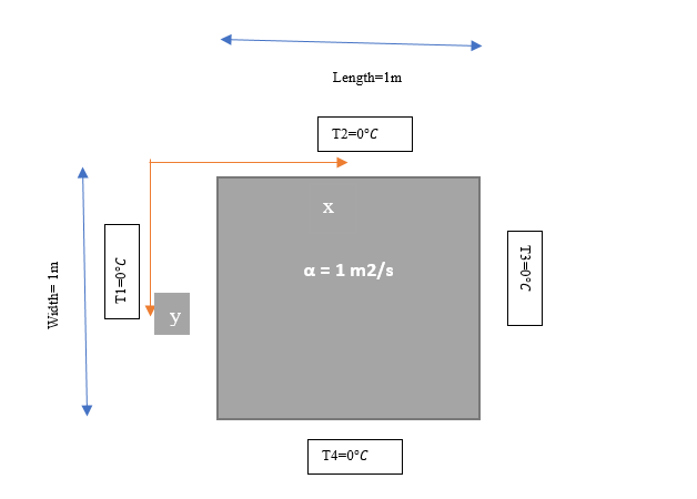
Firstly, we start with analyzing the problem by considering the general heat diffusion equation.

Equation 1

Here it is assumed that material properties do not change at any point along the body. In other words, the body is homogenous. Also, it is assumed that temperature does not vary significantly along the z direction when it is compared with x and y directions. Another thing is that it is assumed that there is no heat generation inside the body. Then for 2D transient heat diffusion with no heat generation, Equation 1 reduces to the following simpler form:

Equation 2

Here initial temperature distribution is accepted as:

Homogeneous Dirichlet boundary conditions are imposed on all boundaries:

Then for determining “T”, Equation 2 needs to be solved. Here Finite Difference Method moves in, helps us to solve that equation. With this method firstly partial derivatives are replaced with the finite difference approximations. So, time derivate is replaced with first order forward difference and the space derivatives are replaced by second order centered difference approximations. Then the Eq.2 becomes the following:

Equation 3

For the sake of simplicity, let Δx = Δy.

Here “i” represents the node location along the x direction, “j” represents the node location along the y direction and “n” represents the time step. Another thing is that since this is an explicit method, temperatures Ti,j’s at future times (n+1) can be directly obtained based on Ti,j’s at present time (n).

2D domain area which has been divided by nodes, has been visualized as in the following figure:

Uniform Grid for 2D Finite Difference Method (41 x 41 Nodes)

Here, there are a total of 1681 (41*41) nodes in total and temperatures are fixed at the boundary nodes. In addition, there are (N-2)² = 39² = 1521 interior nodes, and 1681–1521=160 boundary nodes. Also, grid spacing has been preferred as dx=dy=1/(N-1)=1/40=0.025

The finite difference solver implements a two-dimensional explicit forward time central space (FTCS) scheme for the transient heat equation on the unit square. A uniform Cartesian grid with N nodes per direction dx and dy have been generated and initial condition has been predescribed while zero Dirichlet boundary cnditions are enforced by setting the outer rows/columns to zero. For each time step, the previous solution field (temperature at time step “n”) is copied and only the interior nodes have been updated according to the following formula:

Hence boundary node values remain fixed. The time step “dt” is chosen proportional to dx² (=dy²) for being cautious about the stability constraints of the explicit scheme and is subsequently adjusted so that final time T=1 has been reached exactly. The full transient solution has been stored at each time level with the purpose of post-processing and error evaluation.

Implementation

def fdm_2d(N=41, T=1.0):
    dx = 1/(N-1)
    dt = 0.24*dx**2

The spatial domain is discretized into a uniform Cartesian grid with spacing Δx=Δy. The time step is chosen proportional to Δx² to satisfy the stability condition of the explicit FTCS scheme for the heat equation.

A von Neumann stability analysis shows that, in two spatial dimensions (2D), stability requires [13]:

Choosing Δt= 0.24Δx² ensures numerical stability.

Implementation

The number of time steps is adjusted to ensure that the final simulation time exactly matches “T”. The dimensionless diffusion number “r” controls numerical stability and diffusion strength.

Nt = int(np.ceil(T/dt))+1
    dt = T/(Nt-1)
    r = dt/dx**2
    print(f"FDM: N={N}, r={r:.4f}")

Implementation

A structured tensor-product grid is constructed over the square domain. Such grids are standard in finite difference schemes and allow straightforward stencil-based updates.

x = np.linspace(0,1,N)
y = np.linspace(0,1,N)
X,Y = np.meshgrid(x,y,indexing="ij")

Implementation

The initial condition matches the analytical solution at t=0. Homogeneous Dirichlet boundary conditions are imposed by explicitly setting boundary values to zero at each time step.

This explicit enforcement ensures consistency with the PDE problem solved by the PINN.

U = np.sin(np.pi*X)*np.sin(np.pi*Y)
U[0,:]=0; U[-1,:]=0; U[:,0]=0; U[:,-1]=0

Implementation

The solution is stored at every time step to enable time-resolved error analysis and visualization. Such storage is common in benchmark studies where transient accuracy is examined [13].

U_all = np.zeros((Nt,N,N))
U_all[0] = U.copy()

Implementation

The FTCS scheme discretizes:

• the time derivative using a forward difference,
• the spatial Laplacian using second-order central differences.

The resulting update formula is:

for n in range(1,Nt):
        Un = U.copy()
        U[1:-1,1:-1] = Un[1:-1,1:-1] + r*(
            Un[2:,1:-1] + Un[:-2,1:-1] +
            Un[1:-1,2:] + Un[1:-1,:-2] -
            4*Un[1:-1,1:-1]
        )
        U_all[n] = U

Implementation

Returning the full spatial and temporal grids allows direct comparison with the PINN solution at identical coordinates, enabling fair quantitative and qualitative validation [14].

t_grid = np.linspace(0,T,Nt)
return x, y, t_grid, U_all

6. Physics-Informed Neural Network (PINN)

Physics-Informed Neural Networks (PINNs) are neural networks that incorporate physical laws, expressed as partial differential equations, directly into the training process by embedding them into the loss function, enabling the solution of forward and inverse problems without relying on labeled data.

In the case of solving this 2D Transient Heat Conduction Equation through PINN, PDE won’t be solved and instead, this time PDE will be utilized in computing the loss during the training of the neural network. In particular, the loss is going to be calculated against the derivative of the 2D Heat Conduction equation.

In this study, we have utilized a fully-connected multiplayer perceptron (MLP) with input layer that have 3 features including (x, y, t), 4 hidden layers in which there exists 64 neurons and Tanh activation function applied after each hidden layer. Lastly, in the output layer a single scalar has been produced. Importantly, the network does not represent “u (temperature)” directly, and instead, it represents the following auxiliary function:

Here “teta” denotes the trainable parameters of the neural network.

Implementation

class MLP(nn.Module):
    def __init__(self, layers):
        super().__init__()
        self.layers = nn.ModuleList(
            [nn.Linear(layers[i], layers[i+1]) for i in range(len(layers)-1)]
        )
        self.act = nn.Tanh()

The network weights are initialized using the Xavier (Glorot) normal initialization, which draws parameters from a zero-mean Gaussian distribution with variance scaled according to the number of input and output neurons, a choice shown to facilitate stable signal propagation and efficient training in deep feedforward networks (Glorot & Bengio, 2010) [2].

Xavier initialization has been preferred to stabilize gradients at the beginning of the training. For Tanh networks, Xavier initialization helps keep forward activations and backward gradients from vanishing/exploding early in training, improving optimization stability for MLPs.

Implementation

   for m in self.layers:
       nn.init.xavier_normal_(m.weight)
       nn.init.zeros_(m.bias)

More specifically, for each fully connected layer, the weights are sampled from a zero-mean Gaussian distribution with the following variance:

Where, “n-in” and “n-out” denote the number of input and output neurons of the corresponding layer, respectively.

As a result, the initial weight distributions are fully determined numerically by the layer dimensions (e.g., σ ≈ 0.173 for the 3→64 hidden layer and σ=0.125 for the 64→64 hidden layers). In addition, all bias terms are deterministically initialized to zero. This initialization strategy is particularly important for Physics-Informed Neural Networks employing hyperbolic tangent activation functions, as it preserves variance across layers at initialization and mitigates gradient vanishing or explosion. Consequently, it enables stable computation of higher-order derivatives (such as second order derivative of temperatures in x and y direction) required for enforcing the governing partial differential equation during training.

Forward Propagation in the Multilayer Perceptron

In a feedforward neural network, the forward pass defines how the input features are transformed through successive affine mappings and nonlinear activation functions to produce the network output.

For a multilayer perceptron with L hidden layers, the forward propagation can be written as

Where,

• ϕ(⋅) is a nonlinear activation function (here, hyperbolic tangent),
• the final layer is kept linear to allow the network to represent unrestricted scalar outputs.
• y is the output of the network (scalar temperature)
• h represent the outputs of the hidden layers. It is a kind of hidden representation since it is not physically present inside the code.

Using a linear output layer is particularly important in PINNs, as the network must approximate continuous-valued physical fields rather than bounded classification outputs.

Implementation

 def forward(self, x):
        for layer in self.layers[:-1]:
            x = self.act(layer(x))
        return self.layers[-1](x)

This implementation directly reflects the theoretical formulation:

• self.layers[:-1] iterates over all hidden layers,
• each hidden layer applies an affine transformation followed by a tanh activation,
• the final layer (self.layers[-1]) applies only a linear transformation, with no activation function.

Hard-Constraint PINN Formulation

In this study a hard constraint PINN formulation has been utilized, in which, both initial conditions and boundary conditions have been analytically enforced into the functional form of the solution. Then the final form of the approximate solution obtained from PINN becomes the following [15]:

With initial condition:

At t=0, initial condition can be satisfied exactly,

Also, on the boundary, whether x=0 and x=1 or y=0 and y=1, u(x,y,t) becomes 0. And one can immediately conclude that boundary condition has been enforced analytically for all time.

This hard-constraint construction ensures:

• the initial condition is satisfied exactly
• boundary conditions are enforced by design
• loss function complexity reduces as BC and IC terms drops from loss function

This step is critical for stable and physically meaningful training.

Implementation

class PINN2D_Hard(nn.Module):
    def __init__(self):
        super().__init__()
        self.net = MLP([3, 64, 64, 64, 64, 1])

    def u(self, x, y, t):
        ic = torch.sin(np.pi*x) * torch.sin(np.pi*y)
        v = self.net(torch.cat([x, y, t], dim=1))
        return (1.0 - t)*ic + t*x*(1.0-x)*y*(1.0-y)*v

The function v0(x,y,t) appearing in the hard-constraint ansatz is approximated by a fully connected feedforward neural network. PINN architecture that has been employed in this study can be visualized as the following:

The reason behind selection of four hidden layers with 64 neurons include the following:

• Expressive capacity: Multiple layers enable the network to approximate complex nonlinear functions required to satisfy the PDE residual.
• Smoothness: When combined with the tanh activation function, this depth promotes smooth function representations, which is crucial since second-order spatial derivatives are computed via automatic differentiation.
• Empirical stability: Depth–width combinations of this scale are commonly used in PINN literature as a balance between approximation power and training stability.

In PINN studies, the number of hidden layers and neurons per layer is known to significantly influence solution accuracy and optimization behavior: overly shallow or narrow networks lack sufficient expressive capacity to approximate complex PDE solution, whereas excessively deep or wide networks can suffer from unstable training and poor convergence due to difficulties in minimizing high-order derivative residuals. This trade-off between expressiveness and trainability is discussed in recent PINN literature examining the effects of network architecture on training stability and PDE residual minimization [3]. While 32 neurons may be insufficient to accurately approximate the smooth but nontrivial solution manifold of the 2D heat equation, 128 neurons significantly increase computational cost and can exacerbate optimization difficulties without clear accuracy gains for this problem class.

Compared to the soft-constraint PINNs (the model predicts u directly) that add separate IC/BC penalty terms to the loss, present approach in this study totally eliminates the need to balance such penalties, because the constraints have been encoded in the ansatz itself.

7. Physics-Informed PDE Loss

Since the IC and BC are enforced by construction, training focus on minimizing the residual of the governing PDE.

For PDE residual computation, random points (x,y,t) have been drawn in the domain. Then once, u (temperature) has been computed, Pytorch automatic differentiation has been used to compute ut, uxx, uyy by differentiating the neural network based ansatz u(x,y,t) with respect to inputs (x,y,t). This avoids finite difference approximations for derivatives and is central to the PINN methodology.

Residual error that is going to be minimized at collocation points can be seen as the following:

Implementation

def pde_loss(model, Nf=30000):
x = torch.rand(Nf,1,device=device,dtype=torch.float32,requires_grad=True)
y = torch.rand(Nf,1,device=device,dtype=torch.float32,requires_grad=True)
t = (torch.rand(Nf,1,device=device,dtype=torch.float32,requires_grad=True))**2

Time sampling is biased towards early times to better capture transient behavior.

Automatic differentiation is used to compute derivatives:

Implementation

u = model.u(x,y,t)

    u_t  = torch.autograd.grad(u,t,torch.ones_like(u),True,True)[0]
    u_x  = torch.autograd.grad(u,x,torch.ones_like(u),True,True)[0]
    u_y  = torch.autograd.grad(u,y,torch.ones_like(u),True,True)[0]
    u_xx = torch.autograd.grad(u_x,x,torch.ones_like(u_x),True,True)[0]
    u_yy = torch.autograd.grad(u_y,y,torch.ones_like(u_y),True,True)[0]

The total loss is the mean-squared residual over a set of collocation points:

Implementation

return torch.mean((u_t - (u_xx + u_yy))**2)

The network has been trained by minimizing the PDE residual.

8. Training Strategy: ADAM PRE-TRAINING + L-BFGS Refinement

The parameters of the Physics-Informed Neural Network are optimized by minimizing the physics-based loss function, which measures the mean-squared residual of the governing partial differential equation over a set of collocation points. Let θ denote the trainable parameters of the neural network. The training objective is defined as [4]:

The optimization of trainable parameters “teta” has been performed in two stages. To solve this high-dimensional, non-convex optimization problem, a first-order stochastic gradient-based optimizer has been employed in first place [5].

ADAM Phase

ADAM (Adaptive Moment Estimation) updates the network parameters by combining:

• first-order moment estimates (mean of gradients),
• second-order moment estimates (uncentered variance of gradients).

For each parameter θ_k​, the update rule is given by [6]:

followed by a bias-corrected parameter update. This adaptive mechanism allows different parameters to be updated with different effective learning rates, which is particularly beneficial in PINNs where gradients originating from PDE residuals can vary significantly in magnitude [7].

The model is first trained with ADAM for 8000 epochs. In each training iteration (epoch), the optimizer:

• evaluates the PDE residual over a randomly sampled set of collocation points,
• computes gradients of the loss with respect to all network parameters via automatic differentiation,
• updates the parameters using Adam’s adaptive update rule.

Unlike data-driven learning, this process is entirely physics-driven: no labeled temperature data are required, and the network learns solely by satisfying the governing equation.

The use of a relatively large number of epochs (8000 iterations) allows the optimizer to progressively reduce the PDE residual and move the network parameters toward a region of the parameter space that is suitable for further refinement by second-order optimization methods (e.g., L-BFGS) [8].

In this Pytorch implementation, the loss history has also been stored for later plotting.

Implementation

def train_pinn():
    model = PINN2D_Hard().to(device)

    opt = optim.Adam(model.parameters(), lr=1e-3)
    loss_hist = []

    for ep in range(8000):
        opt.zero_grad()
        loss = pde_loss(model)
        loss.backward()
        opt.step()
        loss_hist.append(loss.item())
        if ep % 500 == 0:
            print(f"[Adam] Epoch {ep}, Loss={loss.item():.3e}")

followed by:

L-BFGS Phase

After ADAM, code applies L-BFGS with a Strong Wolfe line search. L-BFGS is a quasi newton method that approximates second-order curvature information using limited memory of past gradients. This stage is commonly used in PINNs as a refinement step to improve convergence and achieve lower residuals than first order methods alone. This property makes L-BFGS particularly suitable for PINNs, where [4]:

• the loss function involves high-order derivatives of the network output (e.g. u_t, u_xx, u_yy),
• accurate convergence to a low-residual solution is critical,
• full-batch deterministic optimization is preferred over stochastic updates.

The training of Physics-Informed Neural Networks involves minimizing a highly non-convex loss landscape that arises from PDE residuals and their automatic derivatives. First-order optimizers like Adam are good at making robust, large-scale improvements early in training because they adapt learning rates and momentum across parameters, helping escape saddles and poorly conditioned regions of the loss surface. However, first-order methods tend to stall near local minima and may oscillate without fully minimizing the loss. Quasi-Newton methods such as L-BFGS use curvature (approximate second-order information) to accelerate convergence once the parameters are already in a favorable basin. Combining them captures the advantages of both approaches: Adam first broadly explores and reduces large gradients, then L-BFGS fine-tunes for precise convergence and lower PDE residuals [9].

A recent comparative study on PINN training notes that using Adam early helps avoid poor local optima and provides a better starting point for second-order methods, while L-BFGS dramatically improves final loss convergence due to its quasi-Newton updates [10].

lbfgs = optim.LBFGS(model.parameters(), max_iter=400, line_search_fn="strong_wolfe")
    def closure():
        lbfgs.zero_grad()
        loss = pde_loss(model, Nf=15000)
        loss.backward()
        return loss

    t0 = time.time()
    final_loss = lbfgs.step(closure)
    print(f"[LBFGS] Time={time.time()-t0:.2f}s | final loss={final_loss.detach().item():.3e}\n")

    return model, loss_hist

Here, it can be seen that optimizer performs up to 400 quasi-Newton iterations, using a Strong Wolfe line search to ensure sufficient decrease of the loss and stable step sizes. Line search strategies are crucial for second-order methods applied to stiff optimization problems, such as PINN losses dominated by PDE residuals [11].

L-BFGS requires multiple evaluations of the loss and its gradient per iteration to build curvature information. def closure () function provides:

1. a full-batch evaluation of the physics-based loss over collocation points,
2. exact gradients computed via automatic differentiation,
3. a deterministic objective function (no stochastic minibatches).

At the stage of L-BFGS Optimization Step, (starting with final_loss), L-BFGS exploits second-order curvature approximations to rapidly reduce the remaining PDE residual.

Lastly, while reporting execution time and final loss, it can be obviously seen that L-BFGS is more expensive per iteration than Adam but yields substantially lower residual errors, justifying its use as a final refinement step.

9. Error Evaluation Over Time: Absolute L2 Error

To assess the predictive accuracy of the Physics-Informed Neural Network over time, the numerical solution obtained by the PINN is quantitatively compared against the analytical solution. This comparison is performed by evaluating the time evolution of the spatial L²-norm of the error, a standard metric in numerical analysis for time-dependent partial differential equations.

This ensures that all solution fields (PINN, FDM, exact) are evaluated on identical spatial points, eliminating interpolation errors.

Implementation

def time_error_curve(model, U_fdm, t_grid, x, y):
    N = len(x)
    X,Y = np.meshgrid(x,y,indexing="ij")

PINNs operate on point-wise inputs. Flattening the spatial grid converts the 2D field into a batch of N² collocation points, allowing efficient vectorized inference of the neural network solution.

This reflects the continuous functional representation uθ​(x,y,t) emphasized in PINN theory.

Implementation

x_t = torch.tensor(X.reshape(-1,1),dtype=torch.float32,device=device)
y_t = torch.tensor(Y.reshape(-1,1),dtype=torch.float32,device=device)

For comparing PINN solution and analytic solution, at each time t_0 ​, the code forms a constant “t” tensor and computes both u_p (PINN Solution) and u_exact (Analytic Solution) with torch.no_grad() for efficiency (no gradient tracking).

For the FDM solution, FDM solution at that time index is retrieved from U_fdm[i] and converted to torch.

Implementation

pinn_err, fdm_err = [], []

    for i,t0 in enumerate(t_grid):
        t_tensor = torch.full_like(x_t, float(t0))
        with torch.no_grad():
            u_p = model.u(x_t,y_t,t_tensor).reshape(N,N)
            u_e = exact_solution(x_t,y_t,t_tensor).reshape(N,N)
        u_f = torch.tensor(U_fdm[i],dtype=torch.float32,device=device)

As an important notice, at large times (like t=1), the analytical solution decays exponentially:

In such cases, relative error metrics become ill-conditioned. Therefore, all comparisons are performed using the absolute L2 error:

This metric reflects the true physical magnitude of the temperature error. Through the “pinn_err.append”, it has been quantified how well the PINN approximates the true continuous solution at each time level. In addition, through the “fdm_err.append”, difference between Exact solution and the solution obtained from FDM has been evaluated. The FDM error serves as a classical numerical baseline, allowing the PINN’s accuracy to be interpreted relative to a well-understood, grid-based method with known stability and convergence properties.

Implementation

pinn_err.append(torch.norm(u_p-u_e).item())
fdm_err.append(torch.norm(u_f-u_e).item())

Errors are plotted on a logarithmic scale to compare convergence behavior. A semi-logarithmic scale is used because parabolic PDE errors often decay exponentially in time [12].

Implementation

plt.figure(figsize=(8,5))
plt.semilogy(t_grid, pinn_err, label="PINN")
plt.semilogy(t_grid, fdm_err, label="FDM")
plt.xlabel("Time")
plt.ylabel("Absolute L2 Error")
plt.title("Time vs Absolute Error")
plt.grid(True)
plt.legend()

10. Solution Visualization

Beyond scalar error metrics, numerical solvers for partial differential equations are commonly evaluated by visually inspecting the spatial structure of the solution fields at selected time instants. Such qualitative comparisons allow verification that the numerical solution preserves:

• boundary conditions,
• symmetry properties,

In the context of PINNs, visual comparison with classical solvers (e.g., FDM) is particularly important. Consistent color scaling is used to ensure fair visual comparison between PINN and FDM solutions.

The structured grid represents a discrete sampling of the continuous spatial domain. Evaluating all methods on the same grid ensures that observed differences arise from the solver behavior rather than spatial discretization inconsistencies.

Implementation

def plot_solutions(model, U_fdm, t_grid, x, y, t_list=(0.3,1.0)):
    N = len(x)
    X,Y = np.meshgrid(x,y,indexing="ij")

Flattening the spatial grid allows the PINN to be evaluated as a batch of independent query points, reflecting the functional nature of the neural approximation uθ(x,y,t)u_\theta(x,y,t)uθ​(x,y,t).

This is a direct consequence of the PINN formulation introduced by Raissi et al. (2019).

Implementation

x_t = torch.tensor(X.reshape(-1,1),dtype=torch.float32,device=device)
y_t = torch.tensor(Y.reshape(-1,1),dtype=torch.float32,device=device)

Rather than visualizing all time steps, representative snapshots are selected to examine the transient evolution of the solution. This practice is standard in time-dependent PDE analysis, especially for parabolic equations where diffusion smooths the solution over time [12].

Implementation

for t_req in t_list:
        idx = np.argmin(np.abs(t_grid - t_req))

Disabling gradient computation indicates that the model is in inference mode, ensuring computational efficiency and numerical stability. This step confirms that the trained PINN defines a deterministic approximation of the solution field.

Implementation

with torch.no_grad():
    u_p = model.u(x_t,y_t,t_tensor).reshape(N,N).cpu().numpy()

The FDM solution serves as a classical, grid-based benchmark with known stability and convergence properties. Comparing PINN outputs to FDM fields situates the neural solution within established numerical methods.

Implementation

u_f = U_fdm[idx]

Using identical color limits ensures that visual differences correspond to actual magnitude differences rather than plotting artifacts. This is essential for fair qualitative comparison of solution amplitudes.

Implementation

vmax = max(np.max(np.abs(u_p)), np.max(np.abs(u_f)))
vmin = -vmax

This plot illustrates the continuous approximation produced by the PINN, sampled on a structured grid. It allows inspection of smoothness, symmetry, and boundary behavior enforced by the hard constraints.

Implementation

plt.figure(figsize=(6,5))
        plt.imshow(u_p,origin="lower",extent=[0,1,0,1],
                   vmin=vmin,vmax=vmax,aspect="auto")
        plt.colorbar()
        plt.title(f"PINN Solution at t={t0:.3f}")
        plt.xlabel("y"); plt.ylabel("x")

The visualized FDM solution represents the outcome of a classical explicit time-stepping scheme with stability constraints. Its comparison with the PINN solution highlights similarities and differences between grid-based and mesh-free solvers.

Implementation

plt.figure(figsize=(6,5))
        plt.imshow(u_f,origin="lower",extent=[0,1,0,1],
                   vmin=vmin,vmax=vmax,aspect="auto")
        plt.colorbar()
        plt.title(f"FDM Solution at t={t0:.3f}")
        plt.xlabel("y"); plt.ylabel("x")

11. Main Execution Pipeline

The “main” script:

• trains the PINN,
• computes the FDM solution,
• visualizes solutions and errors,
• plots the PINN training loss history.

Implementation

if __name__ == "__main__":
    model, loss_hist = train_pinn()
    x, y, t_grid, U_fdm = fdm_2d(N=41, T=1.0)

    plot_solutions(model, U_fdm, t_grid, x, y)
    time_error_curve(model, U_fdm, t_grid, x, y)

    plt.figure(figsize=(7,4))
    plt.plot(loss_hist)
    plt.title("PINN Training Loss (Adam phase)")
    plt.xlabel("Epoch")
    plt.ylabel("Loss")
    plt.grid(True)

    plt.show()

12. Results

This implementation demonstrates that:

• While the Physics-Informed Neural Network accurately satisfies the governing partial differential equation and imposed constraints, its long-time predictions exhibit small spatial variations, whereas the finite difference method naturally converges to the asymptotic zero solution.
• At early times (t=0.3), PINN accurately reproduces the analytical solution as much as FDM and absolute L2 error values decays the values on the order of 1/10³.
• FDM maintains lower absolute error throughout the simulation.
• PINN error decreases monotonically but stabilizes at further times.
• At late times (t=1), both methods approach zero temperature, but FDM converges more rapidly.

13. What are the advantages of PINNs?

While PINNs can compete with FDM methods in this kind of classical engineering problems, PINNs remain attractive especially for:

• inverse problems with unknown parameters
• sparse or noisy measurement data
• complex or irregular geometries
• problems where mesh generation is difficult

In such cases, classical discretization methods may become impractical.

REFERENCES

[1] Strauss, Walter A. “Partial Differential Equations: An Introduction” (2nd Edition)

[2] X. Glorot and Y. Bengio, “Understanding the difficulty of training deep feedforward neural networks,” in Proceedings of the Thirteenth International Conference on Artificial Intelligence and Statistics (AISTATS), 2010.

[3] Wang, S., Li, B., Chen, Y., & Perdikaris, P. (2024, February 11). Piratenets: Physics-informed Deep Learning with residual adaptive networks. arXiv.org. https://arxiv.org/abs/2402.00326v3

[4] Raissi, Perdikaris, Karniadakis (2019) Physics-informed neural networks: A deep learning framework for solving forward and inverse problems involving nonlinear PDEs

[5] Wang, Yu, Perdikaris (2021) When and why PINNs fail to train: A neural tangent kernel perspective

[6] Kingma & Ba (2015) Adam: A Method for Stochastic Optimization

[7] Krishnapriyan et al. (2021) Characterizing possible failure modes in PINNs

[8] Lu, L., Meng, X., Mao, Z., & Karniadakis, G. E. (2020, February 14). DeepXDE: A deep learning library for solving differential equations. arXiv.org. https://arxiv.org/abs/1907.04502

[9] Hasan, F., Ali, H., & Arief, H. A. (2025, April 30). From mesh to neural nets: A multi-method evaluation of physics informed Neural Network and Galerkin finite element method for solving nonlinear convection–reaction–diffusion equations — International Journal of Applied and Computational Mathematics. SpringerLink. https://link.springer.com/article/10.1007/s40819-025-01904-y?utm_source=chatgpt.com

[10] Urbán, J. F., Stefanou, P., & Pons, J. A. (2025). Unveiling the optimization process of physics informed neural networks: How accurate and Competitive Can Pinns be? Journal of Computational Physics, 523, 113656. https://doi.org/10.1016/j.jcp.2024.113656

[11] Numerical optimization Jorge Nocedal Stephen J. Wright Springer. (n.d.). https://www.ime.unicamp.br/~pulino/MT404/TextosOnline/NocedalJ.pdf

[12] Thomée, Vidar. (2006). Galerkin finite element methods for parabolic problems. 2nd revised and expanded ed. 10.1007/3–540–33122–0.

[13] LeVeque, R.J. (2007) Finite Difference Methods for Ordinary and Partial Differential Equations. SIAM. http://dx.doi.org/10.1137/1.9780898717839

[14] Karniadakis, G.E., Kevrekidis, I.G., Lu, L. et al. Physics-informed machine learning. Nat Rev Phys 3, 422–440 (2021). https://doi.org/10.1038/s42254-021-00314-5

[15] Lagaris, Isaac & Likas, Aristidis & Fotiadis, Dimitrios. (1998). Artificial Neural Networks for Solving Ordinary and Partial Differential Equations. Neural Networks, IEEE Transactions on. 987–1000. 10.48550/arXiv.physics/9705023.

Complete Code

For .py file, please visit https://github.com/barkinozler/PINN-2D-Heat-Conduction.git

import time
import numpy as np
import torch
import torch.nn as nn
import torch.optim as optim
import matplotlib.pyplot as plt

# ======================================================
# SETUP
# ======================================================
device = torch.device("cuda" if torch.cuda.is_available() else "cpu")
torch.manual_seed(0)
np.random.seed(0)

# ======================================================
# ANALYTIC SOLUTION
# ======================================================
def exact_solution(x, y, t):
    return torch.exp(-2*np.pi**2*t) * torch.sin(np.pi*x) * torch.sin(np.pi*y)

# ======================================================
# MLP
# ======================================================
class MLP(nn.Module):
    def __init__(self, layers):
        super().__init__()
        self.layers = nn.ModuleList(
            [nn.Linear(layers[i], layers[i+1]) for i in range(len(layers)-1)]
        )
        self.act = nn.Tanh()
        for m in self.layers:
            nn.init.xavier_normal_(m.weight)
            nn.init.zeros_(m.bias)

    def forward(self, x):
        for layer in self.layers[:-1]:
            x = self.act(layer(x))
        return self.layers[-1](x)

# ======================================================
# HARD-CONSTRAINT PINN
# u = (1-t)*IC + t*x(1-x)y(1-y)*v_theta
# ======================================================
class PINN2D_Hard(nn.Module):
    def __init__(self):
        super().__init__()
        self.net = MLP([3, 64, 64, 64, 64, 1])

    def u(self, x, y, t):
        ic = torch.sin(np.pi*x) * torch.sin(np.pi*y)
        v = self.net(torch.cat([x, y, t], dim=1))
        return (1.0 - t)*ic + t*x*(1.0-x)*y*(1.0-y)*v

# ======================================================
# PDE LOSS
# ======================================================
def pde_loss(model, Nf=30000):
    x = torch.rand(Nf,1,device=device,dtype=torch.float32,requires_grad=True)
    y = torch.rand(Nf,1,device=device,dtype=torch.float32,requires_grad=True)
    t = (torch.rand(Nf,1,device=device,dtype=torch.float32,requires_grad=True))**2

    u = model.u(x,y,t)

    u_t  = torch.autograd.grad(u,t,torch.ones_like(u),True,True)[0]
    u_x  = torch.autograd.grad(u,x,torch.ones_like(u),True,True)[0]
    u_y  = torch.autograd.grad(u,y,torch.ones_like(u),True,True)[0]
    u_xx = torch.autograd.grad(u_x,x,torch.ones_like(u_x),True,True)[0]
    u_yy = torch.autograd.grad(u_y,y,torch.ones_like(u_y),True,True)[0]

    return torch.mean((u_t - (u_xx + u_yy))**2)

# ======================================================
# TRAIN PINN (Adam + LBFGS)
# ======================================================
def train_pinn():
    model = PINN2D_Hard().to(device)

    opt = optim.Adam(model.parameters(), lr=1e-3)
    loss_hist = []

    for ep in range(8000):
        opt.zero_grad()
        loss = pde_loss(model)
        loss.backward()
        opt.step()
        loss_hist.append(loss.item())
        if ep % 500 == 0:
            print(f"[Adam] Epoch {ep}, Loss={loss.item():.3e}")

    lbfgs = optim.LBFGS(model.parameters(), max_iter=400, line_search_fn="strong_wolfe")
    def closure():
        lbfgs.zero_grad()
        loss = pde_loss(model, Nf=15000)
        loss.backward()
        return loss

    t0 = time.time()
    final_loss = lbfgs.step(closure)
    print(f"[LBFGS] Time={time.time()-t0:.2f}s | final loss={final_loss.detach().item():.3e}\n")

    return model, loss_hist

# ======================================================
# 2D FDM (STABLE FTCS)
# ======================================================
def fdm_2d(N=41, T=1.0):
    dx = 1/(N-1)
    dt = 0.24*dx**2
    Nt = int(np.ceil(T/dt))+1
    dt = T/(Nt-1)
    r = dt/dx**2
    print(f"FDM: N={N}, r={r:.4f}")

    x = np.linspace(0,1,N)
    y = np.linspace(0,1,N)
    X,Y = np.meshgrid(x,y,indexing="ij")

    U = np.sin(np.pi*X)*np.sin(np.pi*Y)
    U[0,:]=0; U[-1,:]=0; U[:,0]=0; U[:,-1]=0

    U_all = np.zeros((Nt,N,N))
    U_all[0] = U.copy()

    for n in range(1,Nt):
        Un = U.copy()
        U[1:-1,1:-1] = Un[1:-1,1:-1] + r*(
            Un[2:,1:-1] + Un[:-2,1:-1] +
            Un[1:-1,2:] + Un[1:-1,:-2] -
            4*Un[1:-1,1:-1]
        )
        U_all[n] = U

    t_grid = np.linspace(0,T,Nt)
    return x, y, t_grid, U_all

# ======================================================
# TIME vs ABSOLUTE ERROR
# ======================================================
def time_error_curve(model, U_fdm, t_grid, x, y):
    N = len(x)
    X,Y = np.meshgrid(x,y,indexing="ij")
    x_t = torch.tensor(X.reshape(-1,1),dtype=torch.float32,device=device)
    y_t = torch.tensor(Y.reshape(-1,1),dtype=torch.float32,device=device)

    pinn_err, fdm_err = [], []

    for i,t0 in enumerate(t_grid):
        t_tensor = torch.full_like(x_t, float(t0))
        with torch.no_grad():
            u_p = model.u(x_t,y_t,t_tensor).reshape(N,N)
            u_e = exact_solution(x_t,y_t,t_tensor).reshape(N,N)
        u_f = torch.tensor(U_fdm[i],dtype=torch.float32,device=device)

        pinn_err.append(torch.norm(u_p-u_e).item())
        fdm_err.append(torch.norm(u_f-u_e).item())

    plt.figure(figsize=(8,5))
    plt.semilogy(t_grid, pinn_err, label="PINN")
    plt.semilogy(t_grid, fdm_err, label="FDM")
    plt.xlabel("Time")
    plt.ylabel("Absolute L2 Error")
    plt.title("Time vs Absolute Error")
    plt.grid(True)
    plt.legend()

# ======================================================
# PLOT SOLUTIONS (SAME VMIN / VMAX)
# ======================================================
def plot_solutions(model, U_fdm, t_grid, x, y, t_list=(0.3,1.0)):
    N = len(x)
    X,Y = np.meshgrid(x,y,indexing="ij")
    x_t = torch.tensor(X.reshape(-1,1),dtype=torch.float32,device=device)
    y_t = torch.tensor(Y.reshape(-1,1),dtype=torch.float32,device=device)

    for t_req in t_list:
        idx = np.argmin(np.abs(t_grid - t_req))
        t0 = float(t_grid[idx])
        t_tensor = torch.full_like(x_t, t0)

        with torch.no_grad():
            u_p = model.u(x_t,y_t,t_tensor).reshape(N,N).cpu().numpy()

        u_f = U_fdm[idx]

        vmax = max(np.max(np.abs(u_p)), np.max(np.abs(u_f)))
        vmin = -vmax

        plt.figure(figsize=(6,5))
        plt.imshow(u_p,origin="lower",extent=[0,1,0,1],
                   vmin=vmin,vmax=vmax,aspect="auto")
        plt.colorbar()
        plt.title(f"PINN Solution at t={t0:.3f}")
        plt.xlabel("y"); plt.ylabel("x")

        plt.figure(figsize=(6,5))
        plt.imshow(u_f,origin="lower",extent=[0,1,0,1],
                   vmin=vmin,vmax=vmax,aspect="auto")
        plt.colorbar()
        plt.title(f"FDM Solution at t={t0:.3f}")
        plt.xlabel("y"); plt.ylabel("x")

# ======================================================
# MAIN
# ======================================================
if __name__ == "__main__":
    model, loss_hist = train_pinn()
    x, y, t_grid, U_fdm = fdm_2d(N=41, T=1.0)

    plot_solutions(model, U_fdm, t_grid, x, y)
    time_error_curve(model, U_fdm, t_grid, x, y)

    plt.figure(figsize=(7,4))
    plt.plot(loss_hist)
    plt.title("PINN Training Loss (Adam phase)")
    plt.xlabel("Epoch")
    plt.ylabel("Loss")
    plt.grid(True)

    plt.show()