The GPU Inference Stack: TensorRT, vLLM, Triton, and ONNX Runtime Compared

By Sharat Nellutla — Principal Engineering Manager, Microsoft. All content is original and copyright-protected.

What an inference engine actually does

Inference engines sit between a trained model artifact and the GPU. They take the trained weights, optimize the computation graph, plan memory, pick kernels, and schedule requests. Each engine I work with — TensorRT, vLLM, Triton Inference Server, and ONNX Runtime — handles those steps differently, and most production failures I’ve debugged trace back to a mismatch between the engine’s assumptions and the workload it ended up serving.

This post is the playbook I reach for when picking up serving systems for the first time on a new project. The goal is to be able to design serving systems that integrate multiple engines, diagnose bottlenecks that show up anywhere from kernel launches to allocator behavior, and reason about trade-offs across throughput, latency, memory efficiency, and hardware utilization.

The pipeline is roughly the same across all four. Model ingestion parses formats like ONNX, PyTorch, or TensorFlow. Graph optimization applies layer fusion, constant folding, and precision conversion. Memory planning decides how to reuse activations and (for transformers) how to manage the key-value cache. Kernel selection draws on libraries like cuBLAS and cuDNN or custom CUDA implementations. Runtime scheduling handles dynamic batching, request queuing, and partitioning the GPU across instances.

Each engine emphasizes different parts of that pipeline. TensorRT focuses on optimizing static graphs and calibrating for lower precision formats like INT8 and FP16 to maximize throughput on NVIDIA hardware. vLLM is tailored for transformer models and uses techniques like PagedAttention to manage memory more effectively during variable-length generation. Triton acts as the orchestration layer in front of those backends, providing request routing, dynamic batching, and a uniform API for clients. ONNX Runtime is the most portable of the four — it ships an execution provider abstraction so the same graph can land on CUDA, TensorRT, DirectML, or CPU, which matters when the cluster mixes accelerator generations.

The primary bottleneck depends on the workload. For low-latency, small-batch serving, kernel-launch overhead and PCIe transfer latency dominate, so reducing kernel launches via fusion and minimizing CPU↔︎GPU round trips is essential. For large-batch workloads, memory bandwidth is the limit, and high utilization is what unlocks throughput. With transformers, fragmentation in the KV cache can take a healthy node into out-of-memory territory, which is why memory layout matters as much as the kernels. In multi-tenant serving, dynamic batching is the lever that pushes GPU utilization up — at the cost of tail latency and tighter SLO management.

Inference engine system context

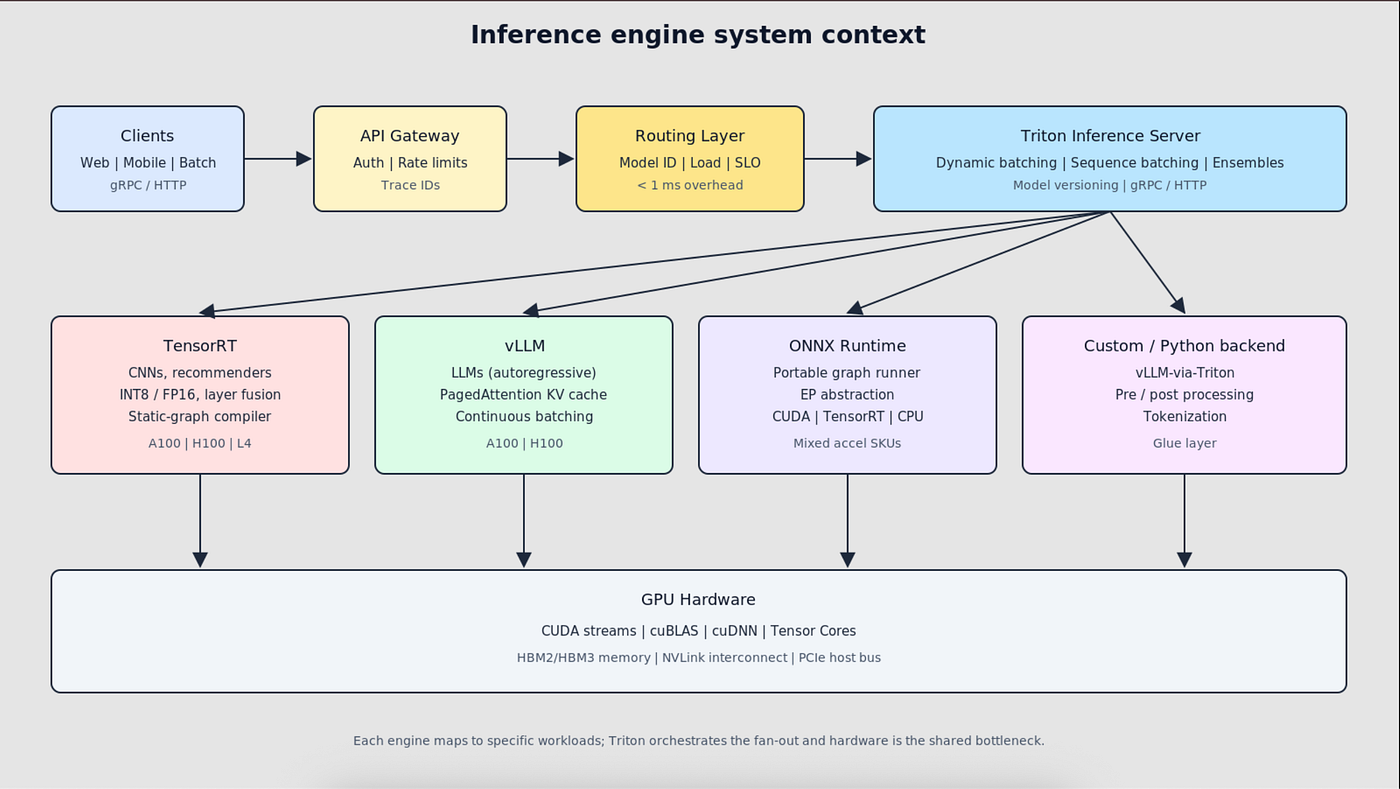
Inference engine system context

Where TensorRT, vLLM, Triton, and ONNX Runtime sit between client requests and the GPU.

The rest of this post walks through each engine in detail — optimization pipelines, memory management, batching, and the production patterns I rely on when deploying them.

How TensorRT compiles a model in three phases

TensorRT is a graph compiler that runs in three distinct phases: parsing, optimization, and runtime execution. Understanding each phase is what lets me predict which fusions will fire, explain calibration-cache behavior, and recognize configuration errors that quietly tank throughput.

During parsing, TensorRT takes a model from formats like ONNX or UFF and constructs an internal intermediate representation (IR) graph. The IR preserves layer semantics while abstracting away framework-specific details. The parser also validates tensor shapes, identifies unsupported operations, and flags dynamic dimension requirements. In production, the parsing errors I see most often come from custom operators without TensorRT plugin implementations, or from shape-inference failures in models that use control flow.

Optimization is where most of the speedup comes from. TensorRT performs layer fusion, selects precision, and autotunes kernels. Layer fusion combines adjacent operations into single CUDA kernels and eliminates the intermediate memory transfers that would otherwise slow execution. TensorRT recognizes patterns like Conv → BatchNorm → ReLU and fuses them into a single kernel, which can cut memory-bandwidth consumption by 60 to 80 percent for typical convolutional neural networks.

During this phase the builder profiles different kernel implementations for each fused layer on the target GPU, measuring latency under different input shapes. For ResNet-50 on an A100, the builder might evaluate 200 to 400 kernel variants per layer to find the ones that minimize overall latency. This profiling is not cheap: builds take 5 to 20 minutes for ResNet-50 and 30 to 90 minutes for larger models like BERT-Large, depending on complexity and how many optimization profiles you’ve configured.

A consequence I want to flag here: the engine you ship to production is the output of a one-time profiling pass against one specific GPU SKU. If you change SKUs, you rebuild. If you change shape profiles, you rebuild. Treat the build step as part of your release pipeline, not as something you re-run by hand under pressure.

TensorRT compile pipeline

Parse → optimize → serialize → runtime: TensorRT’s three phases and the artifacts each produces.

Precision calibration is another critical optimization, especially for INT8 quantization. It requires a representative calibration dataset. TensorRT runs the model in FP32 on 500 to 1000 calibration samples and collects activation histograms for each layer. The calibrator then computes scaling factors that minimize the difference between the FP32 and INT8 distributions. INT8 on BERT-Large delivers 2.5 to 3.5x throughput over FP16 on A100 Tensor Cores — over 8,000 queries per second at batch size 32 — with negligible accuracy degradation.

The final phase is engine serialization, which produces a binary plan file containing the optimized CUDA kernels, the layer execution order, memory allocation strategies, and precision metadata. The serialized engine is tied to a specific GPU architecture: an engine built for A100 will not run on V100. Sizes range from around 50 MB for ResNet-50 to over 2 GB for very large models like GPT-3.

At runtime, TensorRT deserializes the engine, allocates GPU memory for activations and weights, and executes layers in dependency order. The runtime supports CUDA streams, which enables concurrent execution and pipeline parallelism across inference requests. For batch size one on ResNet-50 with FP16, end-to-end latency typically falls in the 2 to 3 millisecond range — a real-world signal that precision reduction and Tensor Cores are pulling their weight.

PagedAttention: applying virtual memory to the KV cache

vLLM’s PagedAttention is one of my favorite ideas in inference: it applies operating-system virtual-memory paging to KV cache, and that one idea is what turns fragmentation from a hard limit into a manageable cost. At production scale, fragmentation is the single biggest constraint on batch size and throughput for LLM serving.

Traditional LLM serving allocates a contiguous chunk of memory for each request’s KV cache up front, sized to the maximum sequence length — often 2,048 or 4,096 tokens. For Llama-2–7B with 32 layers and a hidden dimension of 4,096, each token’s KV cache is 524 KB. A request configured for 2,048 tokens reserves about 1 GB of memory per request. If the actual completion only uses 300 tokens, 85 percent of that allocation sits locked and unavailable. When many variable-length requests run together, memory utilization can collapse to 20 to 40 percent, with out-of-memory failures right behind it.

PagedAttention borrows from OS virtual memory. Instead of contiguous allocation, each sequence’s KV cache is divided into fixed-size blocks — typically 16 tokens, though the block size is tunable. A block manager tracks free physical blocks in GPU memory and maintains a mapping table from logical block indices to physical addresses. When a sequence generates a new token, the manager allocates only the blocks needed: a 300-token sequence uses 19 blocks instead of the 128 blocks a 2,048-token reservation would have required. Physical blocks can be scattered across memory, and the attention kernel uses the mapping table to gather them at compute time.

PagedAttention block layout

Contiguous KV cache versus PagedAttention: blocks plus a block table replace one big reservation.

The kernel itself is what makes this practical. Standard attention multiplies a contiguous query matrix by the transpose of a contiguous key matrix; with PagedAttention, the key matrix is split across non-contiguous physical blocks. The kernel takes a block table that maps logical indices to physical addresses, walks the blocks during the attention loop, gathers keys and values from each block, computes dot products, applies softmax, and writes outputs. The irregular memory access pattern costs about 10 to 15 percent in compute overhead, but the memory savings unlock far larger batches and more than pay for it. On an A100 80 GB with Llama-2–70B at 2,048 context length, naive allocation tops out around batch size 8, while PagedAttention reaches batch sizes of 24 to 32.

Block size is a meaningful tunable. Smaller blocks (4 to 8 tokens) reduce internal fragmentation — the wasted space inside partially filled blocks — but inflate metadata: more block-table entries and more iterations in the kernel loop. Larger blocks (32 to 64 tokens) minimize metadata but waste memory when sequences don’t align to block boundaries. Empirically, 16 tokens hits the right balance: average internal fragmentation is about 8 tokens per sequence, or roughly 4.2 MB of waste for Llama-2–7B — negligible against the hundreds of megabytes saved by avoiding full-context preallocation. A 2,048-token sequence needs 128 block-table entries, which is cheap to cache.

The biggest payoff is continuous batching. New requests can join the batch mid-generation as soon as a slot opens, instead of waiting for the slowest sequence to finish. With contiguous allocation, freed memory often comes back fragmented and unusable until a defragmentation pass — and defrag passes are expensive. PagedAttention returns freed blocks directly to the free list and makes them instantly reusable.

In one workload I look at often — a 70B-parameter model on eight A100s — request-level latency drops from 4.2 seconds with static batching at batch size 8 to 1.8 seconds with continuous batching plus PagedAttention at an effective batch size of 28, holding the throughput target steady. The headline result is more than 2x latency improvement on the same hardware, driven entirely by memory layout — not a faster kernel, not better quantization, just a smarter allocator.

Triton’s request scheduling architecture

Triton Inference Server is the layer that decides how requests are grouped, queued, and dispatched to model instances. The three scheduling primitives I lean on are dynamic batching, sequence batching for stateful models, and ensemble scheduling for multi-model pipelines. The targets I aim for are sub-50 ms p95 latency and 85 percent or better GPU utilization across mixed workloads.

The dynamic batching scheduler is a queue that collects incoming requests and groups them before dispatching to model instances. It exposes two main knobs: max_batch_size, typically 8 to 128 depending on the model’s memory footprint, and preferred_batch_size, usually set to 50 to 80 percent of the max. There’s also a configurable delay, max_queue_delay, which can range from 0 to 10,000 microseconds.

This is the classic latency-versus-throughput dial. A low delay (around 1 ms) prioritizes latency and can hold p95 under 10 ms, but batch fill rates drop to 30 to 50 percent of max_batch_size. Higher delays (5 to 10 ms) push fill rates to 85 to 95 percent at the cost of adding that delay to the latency budget. In practice I configure 2 to 4 ms for user-facing inference and 8 to 10 ms for batch workloads where throughput dominates.

Instance group configuration controls how many parallel processes can serve a single model. Each instance is an independent copy of the model in GPU memory with its own CUDA stream and execution context. With four instances, four batches can execute concurrently, and the scheduler distributes requests across instances using round-robin or least-loaded policies. The number of instances should track the ratio of model inference time to the target latency budget. If a model takes 5 ms to run and you want p95 under 20 ms with a 3 ms batching delay, you need at least two instances to keep the queue from blowing up.

Sequence batching matters for stateful models — conversational AI, video frame processing, anything where requests need ordering. The scheduler tracks per-sequence state and ensures requests from the same sequence run on the same instance in order. A timeout parameter controls how long idle sequences stick around before eviction.

There are two scheduling strategies that matter here. The oldest strategy maximizes throughput by mixing requests from different sequences in the same batch; the direct strategy keeps one sequence per batch to minimize latency. If active sequences exceed instance capacity, latency climbs, so production systems usually implement sequence affinity that routes related sequences to the same instance and avoids context-switch overhead.

Ensemble scheduling chains models in a directed acyclic graph. Each model’s output feeds the next, which enables pipeline parallelism: as soon as a stage finishes a batch, the outputs flow downstream with no extra coordination. Combined with dynamic batching at each stage, ensembles are how I get end-to-end inference pipelines to behave like a tuned production system rather than a stack of independent services.

The interaction between these three schedulers is what makes Triton interesting in production. Dynamic batching alone is fine for stateless models, sequence batching alone handles stateful workloads, but real systems usually have both stateful and stateless models behind the same gateway. Configuring instance groups, queue delays, and ensemble topologies per model is the part of the deployment that takes the most iteration — and the part where most of the latency wins or losses actually come from.

ONNX Runtime execution providers and partition boundaries

ONNX Runtime separates graph optimization and scheduling from the kernels that actually run on each backend through an execution-provider (EP) abstraction. Each EP exposes a GetCapability interface that lists the operators it supports along with type, shape, and attribute constraints. The mental model worth internalizing is that a single CPU-fallback operator on the hot path can cut throughput by 10x to 100x — and the partition algorithm makes that easy to do by accident.

The graph partitioner walks the registered EPs in priority order (configurable by the user) and performs a single-pass greedy assignment: for each node in the graph, it assigns the node to the highest-priority EP that claims to support it. The pass creates contiguous subgraphs that get fused into partitions to minimize data movement between providers. The algorithm is linear in graph size, which is great, but the greediness can produce suboptimal partitions when EPs have overlapping or incomplete coverage.

The TensorRT EP, for instance, converts assigned subgraphs into TensorRT engines via the INetworkDefinition API and applies layer fusion, precision calibration, and kernel autotuning. On transformers like BERT-base, that path can deliver 3x to 8x over the CUDA EP because it fuses multi-head attention into single kernels and uses INT8 quantization with per-channel scales.

The catch is operator coverage. TensorRT 8.x doesn’t support dynamic control-flow operations like If, Loop, or Scan, and it doesn’t cover shape-manipulation ops like NonMaxSuppression or RoiAlign. When unsupported nodes sit on a critical path, they fall back to the CPU EP. That fallback inserts synchronous memory copies before and after the CPU node, which stalls the GPU and drops throughput by 10x to 100x depending on tensor size and PCIe bandwidth.

Partition boundaries cost you in two more subtle ways. First, even when both sides are on GPU, an EP handoff inserts memory copies that hurt latency disproportionately for small batches in online serving — the copy overhead is fixed per handoff, so a 1-sample batch pays the same memory-copy cost as a 32-sample batch but has 32x less compute to amortize it over.

Second, mixed-precision execution across EPs can introduce numerical instability. If TensorRT runs a subgraph in INT8 and hands an INT8 tensor to the CUDA EP expecting FP16, the runtime may insert an implicit Dequantize without preserving the original scale factors, and the accumulated error can exceed acceptable thresholds for the model.

The greediness of the partitioner means EP priority order has a large effect on performance. Putting TensorRT first maximizes GPU utilization, but it can over-partition when TensorRT can’t support some nodes. Putting CUDA first ensures coverage but loses TensorRT’s fusion opportunities. For models I care about, I’ll manually annotate nodes with explicit EP assignments or split the model into multiple ONNX graphs to get deterministic partition boundaries — it adds complexity, but it’s the only way to stop the partitioner from making the wrong call on a quiet operator.

Memory bandwidth is usually the bottleneck

A lot of inference performance work is really memory-bandwidth work. The intuition worth building is: identify which operations are memory-bound, compute arithmetic intensity, and use kernel fusion to cut DRAM traffic.

Start with the A100: 312 TFLOPS in FP16, but memory bandwidth is 1,555 GB/s (2,039 GB/s on the 80 GB SKU). The compute is well ahead of what memory can feed. Take ReLU as the simplest example — each FP16 value needs 2 bytes read and 2 bytes written, so 4 bytes total. At 1,555 GB/s, that supports about 388 billion FP16 values per second. Fully utilizing the GPU’s 312 TFLOPS would require 388 TFLOPS of compute — more than the A100 has. So ReLU runs at roughly 40 percent of peak compute even with perfect access patterns.

Arithmetic intensity formalizes this: it’s FLOPs per byte of memory access. Anything below about 50 FLOP/byte on A100 is memory-bound; above 150 FLOP/byte is compute-bound. Matrix multiply lands at 128 to 256 FLOP/byte (compute-bound). Layer normalization and softmax are typically 0.5 to 4 FLOP/byte (severely memory-bound).

Kernel fusion is the most effective response. Fusing operations into a single kernel collapses DRAM round trips. Consider Conv → BatchNorm → ReLU: the unfused version writes the conv output to memory, reads it for BatchNorm, writes the normalized result, then reads again for ReLU. Fusing all three keeps the intermediates in registers and shared memory and cuts memory traffic from about 1.6 GB to 0.53 GB. TensorRT applies these fusions automatically; you can enable them at engine-build time and verify with the engine introspection commands that show fused layers as single nodes. The latency reduction is real — ResNet-50’s first block drops significantly when the standard fusions fire.

Attention has the same problem at a different scale. Standard attention materializes a matrix that’s quadratic in sequence length, so memory bandwidth dominates. FlashAttention sidesteps that by tiling and processing data in blocks that stay in on-chip SRAM, which produces large measured speedups in practice.

Quantization helps too. INT8 weights halve the bytes moved per inference compared to FP16, which roughly doubles effective bandwidth. You do pay some extra FLOPs to convert INT8 back to FP16 for compute, but that’s well within budget for the workloads I run.

The tool I use to make these calls is a roofline analysis: plot achieved performance against arithmetic intensity, and you can see where an operation sits and whether it’s bound by compute or memory. That tells you whether a fusion or a precision change is going to move the needle, or whether you’re already at the memory wall.

The mental model I keep coming back to is that on modern GPUs, compute is cheap and bytes are expensive. Every optimization that’s worth doing is either moving fewer bytes (fusion, quantization, sparsity) or moving the same bytes more efficiently (tiling, on-chip reuse, better prefetch). Adding more FLOPs to save a DRAM round trip is almost always a winning trade.

Three batching strategies and when each one wins

There are three batching strategies I see in production: static, dynamic, and continuous. Each one optimizes for a different traffic shape, and getting the choice wrong is one of the more expensive mistakes in inference serving.

Static batching processes requests in fixed-size groups. The system waits until a configured number of requests have accumulated — say 32 — before invoking the model. It’s the most efficient when arrival rate is high and predictable, because it maximizes GPU utilization, but it has a structural latency problem. If requests arrive at 100 per second and you batch at 32, the average queue time is around 160 ms, which will violate most user-facing SLAs. Static batching is fine for offline jobs that prioritize throughput; in online serving it’s almost always the wrong default.

Dynamic batching aggregates requests opportunistically within a timeout window. With max_queue_delay set to 5 ms, requests that arrive in that window get batched up to max_batch_size and dispatched immediately. The strategy adapts to traffic shape: during spikes, batches fill quickly and throughput is high; during quiet periods, requests still ship after the timeout. In practice this delivers a 3x to 10x throughput improvement over no-batching while holding p99 latency under 20 ms. Sizing the timeout is the only really delicate part — Little’s Law (queue length = arrival rate × wait time) is the relationship I use to pick a defensible value.

Continuous batching is the strategy that matters for autoregressive models. Traditional batching waits for every sequence in a batch to finish before starting a new one. With variable-length outputs, that means the GPU sits idle as the shorter sequences finish, and utilization can fall to 40 to 60 percent. Continuous batching operates at the iteration level: when any sequence finishes, a new request slots in immediately, and the batch stays full throughout execution. The wins are concrete — time-to-first-token drops, sustained throughput rises, and the GPU stays occupied even with extreme length variance.

The picking heuristic is straightforward. Static batching is for offline throughput jobs. Dynamic batching is the default for stateless online inference. Continuous batching is for any autoregressive workload where sequence length is unpredictable.

The choice has a much bigger blast radius than people expect. Picking the wrong batching strategy is one of the most common reasons a system that looked great in benchmarks falls over in production: a model that runs at 5 ms in isolation can show p99 of 200 ms once real traffic hits, because static batching is queueing requests behind a slow batch fill.

Routing across multiple engines in production

Real inference platforms run multiple engines side by side. In the deployments I’ve worked on, that means CNNs for image classification on TensorRT, transformers for embeddings on ONNX Runtime, and LLMs for text generation on vLLM, all behind a single API surface. The routing layer is what makes that work, and I hold it to sub-1 ms overhead and zero-downtime updates.

The routing layer sits between the API gateway and the engine pods. For each request, it picks an engine in under a millisecond based on the model ID, request metadata, current cluster load, and SLO requirements. Triton Inference Server is the unified front I default to because it speaks to TensorRT, ONNX, PyTorch, and vLLM (via its Python backend) over a consistent gRPC or HTTP API, with model versioning and ensemble pipelines built in.

The foundational mechanism is model-specific routing: a routing table that maps model IDs to engine types. A request for ResNet-50 lands on TensorRT pods running on A100s in FP16. A request for BERT-base lands on ONNX Runtime on T4 GPUs with dynamic batching. A request for Llama-70B lands on vLLM on H100 clusters with PagedAttention. The routing layer consults a config service — etcd, Consul, or Kubernetes ConfigMaps — to resolve mappings and health-check endpoints, and for latency-critical paths it caches the mapping in-process with a 5 to 10 second TTL and a watch-based invalidation.

A/B testing and canaries need precision splitting and good observability. A common shape is 95 percent of traffic to a stable TensorRT backend, 5 percent to a candidate ONNX Runtime backend for the same model. The routing layer injects trace IDs and engine-version labels into request metadata, which flow through distributed tracing (Jaeger or Tempo) and metrics (Prometheus). The metrics I watch are p50 and p99 latency, error rate, and throughput. If the candidate holds p99 within 10 percent of baseline and error rate stays under 0.1 percent over 24 hours, it gets promoted. Traffic splitting uses consistent hashing on request IDs so the same user keeps hitting the same backend version through the test.

Fallback chains handle saturation and failure. A three-tier fallback for LLM serving might be: primary vLLM with a p99 target under 200 ms, secondary TensorRT-LLM with a p99 target under 500 ms, tertiary ONNX Runtime on CPU with a target under 2 seconds. The routing layer watches queue depth and response times and shifts traffic between tiers based on configured thresholds.

Cost optimization is the last lever. The router can send small-batch requests (1 to 4 samples) to CPU-based ONNX Runtime pods while routing larger batches (16 or more) to GPU-based TensorRT pods. CPU inference is cheaper at small batch sizes; GPU wins at larger batches because parallelism amortizes the per-request cost. During off-peak hours the system can drain GPU pods entirely and serve from CPU, then warm GPUs back up ahead of the next peak — which requires predictive autoscaling so the GPU instances are ready before load arrives.

Designing a 100k QPS multi-model platform

When I design a serving platform, I start from the bottlenecks and work backward — not from a feature list. The exercise that forces good habits looks like this: design a multi-model serving platform that handles 100,000 QPS across 50 models, holds p99 latency under 100 ms, and runs on 100 A100 GPUs. Models range from 10 MB to 2 GB. Traffic is Zipfian — the top five models absorb 60 percent of requests.

The architecture I’d build uses Triton Inference Server as the orchestration layer. Vision and recommendation models use the TensorRT backend. Transformer NLP models use vLLM for dynamic batching on long sequences.

Per-GPU load is roughly 1,000 QPS on average, but the Zipfian distribution means I can’t allocate uniformly. The hot models get dedicated GPU pools. Replicating each hot model three times and allocating roughly 15 GPUs per hot model gives me the headroom to absorb traffic spikes for the top five. Continuous batching at batch sizes of 32 to 64 amortizes kernel-launch overhead and pushes throughput.

The cold models — the long tail of 45 — share a separate pool of about 25 GPUs. Cold models load on demand, and I budget for a 50 to 100 ms model-swap latency on the first request after eviction. TensorRT’s fusion and INT8 quantization are what get the CNNs to the 1,000-QPS-per-GPU target on the dedicated pool.

The failure mode I care most about on the shared cold pool is memory fragmentation. Concurrent loads of cold models with different memory footprints will produce OOMs, even at moderate utilization. The mitigation is Triton’s model instance groups: pre-allocate memory pools sized for known model classes and cap cold-model requests at about 10 percent of GPU capacity so the shared pool can’t be saturated by a single noisy neighbor.

For p99 latency, the leading indicator I track is batch-formation time inside Triton’s dynamic batcher. If queue depth exceeds 128, I trigger horizontal autoscaling and add GPU replicas. That kicks in before the latency target moves, which keeps the SLO defensible during traffic spikes.

The principle worth internalizing here is the inversion: don’t design around features; design around bottlenecks. Memory bandwidth, compute utilization, and operational surface area are the constraints that drive engine choice and topology, not the other way around.

The architecture above is not the only valid answer. You could swap Triton for a custom router, replace the cold pool with autoscaling per-model deployments, or push everything onto fewer larger GPUs like H100s. The point isn’t the specific shape — it’s that the shape is defensible against the constraints, and that each piece of the topology maps to a quantified bottleneck rather than a habit.

Diagnosing a vLLM throughput regression

The diagnostic skill that matters most in inference work is reasoning past surface metrics — down to resource contention, fragmentation, kernel-level effects, and the failure modes that only show up under sustained load. Here’s a scenario I keep coming back to as a reference test.

A vLLM deployment serving Llama-2–70B on eight A100s has been stable for hours. After six hours, aggregate throughput drops sharply — from 1,200 tokens per second to 300 tokens per second. nvidia-smi reports GPU utilization is still 85 to 90 percent. Requests are queuing up. How do you diagnose this?

The first thing I check is memory fragmentation. nvidia-smi dmon with the memory-usage flag shows how allocation evolves over time — not just headline usage, but how the allocator is fragmenting it. vLLM’s PagedAttention uses a block-based KV cache allocator. After hours of variable-length requests, the allocator can fragment even when total free memory looks healthy. Fragmentation causes allocation failures, which force expensive defragmentation or downward batch-size adjustments — both of which crater throughput while compute utilization stays high.

Next I’d profile with nsys to check whether kernel-launch latency has crept up. Under memory pressure, CPU-scheduling-to-GPU-execution context switches can grow from microseconds to milliseconds, which compounds the throughput problem.

The vLLM metrics themselves are the third leg. Look at the batch-size distribution — if the scheduler is forming smaller batches because the allocator can’t satisfy block requests, throughput drops proportionally while utilization stays high. That gap between utilization and effective throughput is the signal that “GPU is fine” is the wrong conclusion.

Concretely, in the scenario above I’d expect the diagnostic stack to show three correlated signals. nvidia-smi dmon shows a spike in memory allocation rate around the six-hour mark, with fragmentation rising from about 5 percent to about 35 percent. nsys shows kernel-launch gaps widening from roughly 50 microseconds to 2 milliseconds. vLLM’s internal metrics show KV-cache block allocation failures climbing from zero to several hundred per minute, and the active batch size dropping from 128 to around 32. Any one of those signals on its own is suggestive; all three together point unambiguously at allocator fragmentation.

Throughput-regression diagnostic stack

Timeline of throughput vs. fragmentation, plus the three-layer diagnostic stack (nvidia-smi dmon, nsys, vLLM metrics) that pinpoints the cause.

The immediate mitigation is a service restart, which resets the allocator and clears fragmentation. The durable fix is tuning vLLM’s block size and gpu_memory_utilization target. Dropping the default from 0.9 to 0.85 leaves about 10 to 15 percent headroom that the allocator uses to recover from fragmentation. In production I also schedule proactive restarts every 12 to 24 hours so fragmentation never reaches the regression point.

The weak version of this answer is to point at GPU utilization as proof the system is healthy, or to add GPUs without understanding the allocator behavior. Both miss the key distinction: compute utilization is not effective throughput. Memory fragmentation, kernel-launch overhead, and batch-formation behavior are where the actual signal lives.

© 2026 Sharat Nellutla — Principal Engineering Manager, Microsoft. All content is original and copyright-protected.