Electric Vehicle Charging Decision using Dynamic Programming

A hands-on walkthrough of modeling sequential charging decisions under battery constraints

In the last two articles, we explored Dynamic Programming (DP) as a tool for solving Operations Research problems. We discussed how to recognize problems that are well suited for DP, how to decompose them into stages, states, and decisions, and how to model them effectively. We understood the limitations of DP in large-scale settings and work arounds used in practice to manage them. We also worked through a foundational example by modeling the classic Knapsack Problem.

[embed]Dynamic Programming for Large Scale Optimization A practical guide to overcoming DP limitations in real-world applicationsmedium.com

In this article, we move to slightly more complex and operationally meaningful problem. We apply the same DP building blocks to a simplified, but representative, Electric Vehicle (EV) Charging Problem, illustrating how real-world operational decisions can be structured as a sequential optimization problem.

Specifically, this article explains how EV charging decisions can be modeled as a Dynamic Programming problem, shows how feasibility constraints such as battery limits are naturally handled within a DP framework and walks through a complete DP formulation including stages, states, actions, transitions, and cost functions. It then demonstrates a Python implementation for both finding a feasible charging strategy and extending it to explicitly minimize total cost. Along the way, the example highlights why charging earlier than strictly necessary can sometimes reduce overall cost, even when such decisions appear suboptimal from a local perspective.

Problem Overview

An Electric Vehicle (EV) must serve a fixed sequence of customers along a predefined route. The order of customers cannot be changed, but the vehicle may need to detour to charging stations if its battery level is insufficient to continue.

This situation arises in practice when a fleet includes a mix of conventional vehicles and EVs with different battery capacities, and frequently redesigning routes is undesirable.

Each decision affects not only the immediate cost but also feasibility of future actions. There is a clear trade-off between:

• Short-term cost (detouring to charge) and
• Long-term feasibility (avoiding battery depletion)

This is a classic sequential decision-making problem, making it a natural candidate for Dynamic Programming.

While the problem could be formulated as a large mixed-integer optimization model, doing so would introduce unnecessary complexity. Since the route is fixed and only charging decisions need to be optimized, DP offers a much cleaner and more interpretable approach.

Rather than solving a full routing or scheduling problem, the EV charging task can be framed as a sequence of local decisions: Should the vehicle proceed to the next customer, or detour to recharge?

Problem Setup

Consider a vehicle that starts and ends at a base location (node 0) and must serve a fixed sequence of customers numbered from 1 to 9, N={0,1,2,…,9}.

The vehicle follows a predetermined route 0 → 1 → 2 → … → 9 → 0 with no re-routing allowed.

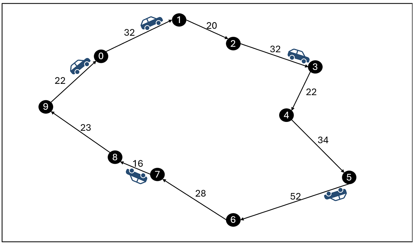
Vehicle Route

Along the route, a small number of charging stations are available at known locations, Q = {1,2,3}.

The following distances are assumed to be known:

• dist_next(n) : distance between customer n and the next customer on the route
• dist(n,q) — distance between customer n and charging station q

Charging Network

The vehicle has a limited battery capacity and consumes energy in proportion to the distance traveled. If the battery level becomes too low, the vehicle must detour to a charging station before continuing.

At each customer node, the vehicle faces a simple decision:

• Continue to the next customer, or
• Detour to a charging station before proceeding.

To keep the example focused, we make the following simplifying assumptions:

• Energy consumption is deterministic, with rate r per unit distance
• Charging always restores the battery to full capacity B_max
• The battery level must never fall below a minimum threshold B_min

In the sections that follow, we model this problem using a dynamic programming framework. We define the stages, states, actions, and transition functions, and demonstrate how this formulation leads naturally to an efficient and interpretable solution.

To build intuition step by step:

1. We first solve a simplified version of the problem that focuses only on feasibility.
2. Once a feasible strategy is established, we extend the model to explicitly minimize total cost.

Dynamic Programming Formulation

1. Stage:

Each customer visit represents a stage in DP. At every stage, the vehicle decides whether to continue to next customer or to charge before proceeding.

2. State:

The state is defined as:(n,b) where,

• n= current customer index
• b = remaining battery level

This state captures all the information needed to make the next decision. Once the current location and battery level are known, past history is irrelevant.

3. Action:

At each state, the vehicle has two possible actions:

1. Continue to the next customer (action = 0)
2. Visit a charging station before continuing (action = nearest charging station to n)

The second option is only feasible if the vehicle has enough battery to reach the charging station.

4. Transition function:

If the vehicle is in state (n,b):

If the vehicle continues without charging, the state transitions as:

(n,b)→(n+1,b−r⋅dist_next(n))

If the vehicle visits charging station q, the next state is:

(n,b)→(n+1,B_max⁡−r⋅dist(n+1,q))

Transitions are allowed only if the resulting battery level remains above B_min.

5. Cost Function:

The total cost includes both transportation and charging costs:

Let:

• c_t: cost per unit distance
• c_f: fixed cost of charging
• c_v​: cost per unit of energy charged

If the vehicle continues from State (n,b) without charging, the value function is:

V(n,b) = c_t⋅dist_next(n) + V(n+1, b- dist_next(n))

If the vehicle charges at charging station q, the cost includes both travel and charging:

cost = c_t⋅[dist(n, q)+ dist(n+1,q)] + c_f + c_v⋅(B_max- (b-r⋅dist(n,q))

and the corresponding value function is:

V(n,b) = cost+ V(n+1, B_max — r⋅dist(n+1,q))

This formulation naturally leads to a recursive DP relation: the cost of being at location n with battery level b depends on the optimal cost of the subproblem at location n+1, with the battery level resulting from the chosen action.

Solution Approach

Although this problem can be modeled as a mixed-integer optimization problem, Dynamic Programming is a better fit for several reasons:

• The route is fixed
• Only charging decisions need to be optimized
• Only a subset of battery levels is reachable
• Sequential feasibility constraints are handled naturally

A top-down DP is particularly effective here. Only states that are actually reachable are evaluated, which keeps computation manageable even when battery levels are discretized.

An important benefit of this approach is that infeasible paths are handled naturally. If the vehicle cannot reach a charging station from a given customer, the recursion backtracks and adjusts earlier decisions without explicit constraint handling.

Python Implementation: Greedy decisions

The first implementation focuses on feasibility rather than cost optimality. The algorithm behaves like a Greedy DP with backtracking:

• Move forward without charging when possible
• If infeasible, attempt to charge
• If charging is also infeasible, backtrack and revise earlier decisions

This guarantees a feasible route whenever one exists.

The following implementation shows how the EV charging problem can be set up as a Dynamic Programming Model.

Step 1: Inputs

We begin by defining the key inputs that describe the problem.

NUM_CUSTOMER_LOCATIONS = 10
NUM_CHARGING_STATIONS = 3
BATTERY_MAX= 95
BATTERY_MIN = 10
RATE_OF_CONSUMPTION = 0.5 # units of battery consumed per unit distance
# Charging cost parameters
FIXED_CHARGING_COST = 2.0  # fixed cost per charge
VARIABLE_CHARGING_COST = 0.5  # cost per unit battery charged
TRAVEL_COST_PER_UNIT_DISTANCE = 0.2  # cost per unit distance traveled

cust = [i for i in range(NUM_CUSTOMER_LOCATIONS+1)]
route = cust + [cust[0]]  # circular route
dist_Matrix = [[35,76,32],
               [22,72,38],
               [18,56,44],
               [38,42,56],
               [32,24,48],
               [74,32,54],
               [72,28,46],
               [68,34,22],
               [48,46,18],
                [55,86,34]]
route_distances = [32, 20, 32, 22, 34, 52, 28, 16, 23, 22]  # distances between consecutive customers in the route

Step 2/3: Initialize State and DP Storage

The state is defined by:

• Current location
• Current battery level

The vehicle starts at location 0 with a full battery.

The dp_array dictionary stores:

• The action taken at each state
• The cumulative cost up to that point

This is required to trace the entire solution after DP is solved.

#2. Initialize States
state = {}
state[0] = {0: {'loc': 0, 'battery': BATTERY_MAX}}  # initial battery level at start location

#3. Initiate DP array, stores action and cumulative cost for each state
dp_array = {}

Step 4: Define helper functions

These functions simplify the DP logic and make the code easier to follow.

#4. Define helper functions

#4.1 Identify the nearest enroute station between current and next location
def get_closest_station(loc_idx):
    total_dist = [a + b for a, b in zip(dist[route[loc_idx]], dist[route[loc_idx+1]])]
    dist_to_closest_station = min(total_dist)
    closest_station = total_dist.index(dist_to_closest_station)
    return closest_station

#4.2 Get distance either from current customer to next or customer to charging station
def get_dist(loc_idx, station_idx = None):
    if station_idx is None:
        return route_distances[loc_idx]
    return dist[route[loc_idx]][station_idx]

#4.3 Compute travel cost 
def get_travel_cost(loc_idx, station_idx = None):
    return TRAVEL_COST_PER_UNIT_DISTANCE * get_dist(loc_idx, station_idx)

#4.4 Compute charging cost
def get_charging_cost(battery_before):
    charged_units = BATTERY_MAX - battery_before
    return FIXED_CHARGING_COST + VARIABLE_CHARGING_COST * charged_units

#4.5 Compute total cost based on action
def get_total_cost(loc_idx, station_idx = None, battery_cur = None):
    if station_idx is None:
        return get_travel_cost(loc_idx)
    else:
        travel_cost = get_travel_cost(loc_idx, station_idx) + get_travel_cost(loc_idx+1, station_idx)
        battery_before = battery_cur - get_battery_consumption(loc_idx, station_idx)
        charging_cost = get_charging_cost(battery_before)
        return travel_cost + charging_cost

#4.6 Compute battery consumption when covering distance
def get_battery_consumption(loc_idx, station_idx = None):
    return RATE_OF_CONSUMPTION * get_dist(loc_idx, station_idx)

#4.7 Compute battery level at next location if current action is taken
def get_battery_at_next(battery_cur, loc_idx, station_idx = None):
    return battery_cur - get_battery_consumption(loc_idx, station_idx)

#4.8 Update DP array to include action and cumulative cost for current state
def update_dp_array(loc_idx, battery_cur, action, cum_cost):
    dp_array[(route[loc_idx], battery_cur)] = (action, cum_cost)

NOTE : Writing the helper functions separately improves clarity by keeping the DP logic focused on decisions and state transitions rather than low-level calculations. It makes the code easier to read, debug, and verify against the underlying DP formulation, while also allowing cost or battery models to be changed or extended without modifying the core algorithm.

Step 5: DP Recursion

As we want to find a feasible route, unlike a classical DP that evaluates all actions, this implementation behaves like a greedy DP with backtracking, where we “follow the cheapest path forward; if you hit a dead end, step back and fix the mistake”.

NOTE: For a full DP that evaluates all decisions (instead of this heuristic), skip this and see DP Recursion in next section.

The DP recursion performs following steps:

1. Base Case: If the vehicle has reached the final location, no further decisions are required and the recursion terminates.
2. Greedy Forward Move: The algorithm first computes the battery level after moving to the next location without charging. If the battery remains above the minimum threshold and the algorithm is not backtracking, the vehicle continues forward and no alternative action is explored.
3. Decide to Charge on failure: If the battery is insufficient to reach the next location, or if the recursion is in a backtracking phase, the algorithm considers charging at the closest enroute charging station between the current and next customer locations.
4. Check charging feasibility: If the vehicle has enough battery to reach the charging station, it detours to the station, charges to full capacity, and then proceeds to the next location.
5. Backtrack: If the charging option is also infeasible, the algorithm backtracks one step, restores the previous battery level and cumulative cost, and sets the last_fail flag. This forces a charging decision at an earlier location in the subsequent recursion.

Backtracking allows the algorithm to recover from infeasible greedy decisions and ensures feasibility without explicitly modeling battery constraints in the DP state.

DP Recursion with Greedy Decision and Backtracking

The code implementing this is given below:

#5. Define DP function
# location index, current battery level are used to define state
# cumulative cost is used to track and store total dp costs
# track previous cost and battery level to backtrack in case of infeasibility
# use last_fail flag to identify backtrack scenario
def dp(loc_idx, battery_cur, battery_prev, cost_cum, cost_prev, last_fail = 0):

    if loc_idx == len(route)-1:
        update_dp_array(loc_idx, battery_cur, None, cost_cum)
        return 0

    battery_next = get_battery_at_next(battery_cur, loc_idx, station_idx = None)
    if battery_next > BATTERY_MIN and not(last_fail):
        cost =  get_total_cost(loc_idx)
        update_dp_array(loc_idx, battery_cur, "Next", cost_cum + cost)
        return cost + dp(loc_idx+1, battery_next, battery_cur, cost_cum + cost, cost)

    if battery_next<= BATTERY_MIN or last_fail:
        closest_station = get_closest_station(loc_idx)
        battery_to_station = get_battery_consumption(loc_idx, closest_station)

        if battery_cur - battery_to_station >= BATTERY_MIN:
            battery_next = get_battery_at_next(BATTERY_MAX, loc_idx+1, closest_station)
            cost = get_total_cost(loc_idx, closest_station, battery_cur)
            update_dp_array(loc_idx, battery_cur, closest_station+1, cost_cum + cost)
            return cost + dp(loc_idx+1, battery_next, battery_cur, cost_cum + cost, cost)
        elif battery_cur - battery_to_station < BATTERY_MIN:
            if last_fail:
                # If solution fails again during backtrack, no feasible solution
                print("No feasible solution")
                return -10000
            return  dp(loc_idx-1, battery_prev , battery_prev, cost_cum - cost_prev, 0 ,1)

Step 6: Solving the Problem

Solve the problem by calling the dp function. The DP starts from the first customer with a full battery.

#6. Solve DP
dp(0, BATTERY_MAX, BATTERY_MAX,0, 0)

Step 7: Output

The final output shows:

• Each visited state
• The action taken
• Cumulative cost

This provides a complete and interpretable charging strategy.

#7. Print dp array to see final solution
for state in dp_array:
    print(f"State: {state}, Action: {dp_array[state][0]}, Cost: {dp_array[state][1]}")

In the final output, the total cost is 139, and charging decisions appear only at locations 4 and 8, exactly where continuing without charging would cause the vehicle to run out of battery . This ensuring feasibility while keeping charging stops to a minimum.

State: (0, 95), Action: Next, Cost: 6.4
State: (1, 79.0), Action: Next, Cost: 10.4
State: (2, 69.0), Action: Next, Cost: 16.8
State: (3, 53.0), Action: Next, Cost: 21.2
State: (4, 42.0), Action: 2, Cost: 66.9
State: (5, 79.0), Action: Next, Cost: 77.3
State: (6, 53.0), Action: Next, Cost: 82.9
State: (7, 39.0), Action: Next, Cost: 86.1
State: (8, 31.0), Action: 3, Cost: 135.0
State: (9, 78.0), Action: Next, Cost: 139.4
State: (0, 67.0), Action: None, Cost: 139.4

Minimizing Total Cost

In the next step, we use dynamic programming recursion to explicitly minimize the overall cost of the solution. The approach discussed so far works well for ensuring feasibility, but it does not actively compare alternatives to find the lowest-cost option.

To achieve cost minimization, we must account for the cost impact of each decision i.e. whether the vehicle continues to the next customer or detours to a charging station at every stage.

Although, in principle, the battery level can vary between minimum and maximum values, only a small and predictable subset of battery levels is actually reached due to deterministic energy consumption. As a result, the same top-down DP approach can still be used without enumerating the full battery range.

The modified DP recursion explicitly evaluates both actions at each stage, propagates cumulative costs forward, penalizes infeasible decisions, and ultimately reconstructs the minimum-cost feasible solution.

Step 4: Modified helper function

Before updating the DP function, we also need to keep track of all battery levels encountered by the vehicle at each location. This requires tracking the states and corresponding information in greater detail than before. For a given location, different actions (and past actions) can result in different starting and ending battery levels, each with its own cumulative cost. To support this, we extend the dp_array structure and update the corresponding helper function so that all such state–action–battery combinations are properly recorded.

#4.8 Update DP array to include action and cumulative cost for current state
def update_dp_array(loc_idx, battery_info, action, cost):
    if loc_idx not in dp_array:
        dp_array[loc_idx] = {}
    if action not in dp_array[loc_idx]:
        dp_array[loc_idx][action] = {battery_info: cost}
    else:
        dp_array[loc_idx][action].update({battery_info: cost})

Modified Step 5: DP Recursion

The new DP recursion follows these steps:

1. Base case: If the vehicle has reached the final location, the recursion terminates. Any remaining battery is penalized through a terminal charging cost.
2. Cost propagation from previous stage: If the last decision involved charging, the same battery level at the current location may be reached through multiple paths, each with a different cost incurred before charging. To handle this, the algorithm identifies the minimum cost of reaching the charging station and updates the cumulative cost accordingly. This ensures that only the best-known cost is propagated forward in the recursion.
3. Action loop: At each location, the algorithm evaluates two possible actions i.e. continuing to the next customer without charging, or detouring to the closest enroute charging station and charging before proceeding.
4. Action 1 — Skip charging: If the vehicle skips charging, the battery level at the next location is computed. If the battery remains above the minimum threshold and the recursion proceeds to the next location.
5. Action 2 — Charging decision: If the vehicle chooses to charge, the algorithm checks whether the current battery level is sufficient to reach the closest charging station. If feasible, the vehicle detours to the station, charges to full capacity, and continues to the next location with an updated battery level.
6. Infeasible charging: If at any step, the vehicle does not have sufficient battery to reach next customer or charging station after following a particular path, the corresponding action is marked infeasible by assigning a large penalty cost.

By explicitly evaluating both actions at each stage and propagating cumulative costs forward, this DP recursion systematically explores feasible routing and charging decisions and identifies the minimum-cost solution without requiring explicit enumeration of all battery states.

DP Recursion for Minimizing Cost for EVCP

Here is the python implementation for above function:

#5. Define DP function
# location index, current battery level are used to define state
# cumulative cost is used to track and store total dp costs
# track previous action to backtrack actions 
def dp(loc_idx, last_action, battery_cur, cost_cum):

    if loc_idx == len(route)-1:
        cost = battery_cur*VARIABLE_CHARGING_COST
        update_dp_array(loc_idx, (last_action,battery_cur, battery_cur), None, cost_cum+ cost)
        return cost_cum + cost

    if last_action != 0:
        for tmp_action in dp_array[loc_idx-1]:
            if tmp_action != 'Next':
                cost_cum = min(dp_array[loc_idx-1][tmp_action].values())
    closest_station = get_closest_station(loc_idx)
    for a in [0,closest_station+1]:
        if a == 0:
            battery_next = get_battery_at_next(battery_cur, loc_idx, station_idx = None)
            if battery_next > BATTERY_MIN:
                cost =  get_total_cost(loc_idx)
                update_dp_array(loc_idx, (last_action,battery_cur, battery_next), "Next", cost_cum + cost)
                #return cost + dp(loc_idx+1, battery_next, cost_cum + cost)   
                dp(loc_idx+1, a, battery_next, cost_cum + cost)
            else:
                update_dp_array(loc_idx, (last_action,battery_cur, battery_next), "Next", 10000)
        else:
            battery_to_station = get_battery_consumption(loc_idx, closest_station)
            battery_next = get_battery_at_next(BATTERY_MAX, loc_idx+1, closest_station)
            if battery_cur - battery_to_station >= BATTERY_MIN:
                cost = get_total_cost(loc_idx, closest_station, battery_cur)
                update_dp_array(loc_idx, (last_action,battery_cur, battery_next), closest_station+1, cost_cum + cost)
                #return cost + dp(loc_idx+1, battery_next, cost_cum + cost)
                dp(loc_idx+1, a, battery_next, cost_cum +cost)
            else:
                update_dp_array(loc_idx, (last_action,battery_cur, battery_next), closest_station+1, 10000)

Extra Step: Reconstructing final solution

The costs corresponding to each state are stored in the dp_array in the previous step. Once we have this, we need to reconstruct the final solution from dp_array.

The following code reconstructs the optimal solution by backtracking through the DP table from the final location to the start.

• It begins by selecting the minimum-cost battery transition at the last location and records the corresponding final battery level.
• Moving backward, it only considers transitions that lead to the previously selected battery level, ensuring battery consistency across stages.
• At each location, the action with the lowest cumulative cost among feasible transitions is chosen and stored, resulting in a cost-optimal and battery-feasible sequence of decisions.

last_battery = None
solution = {}

for n in range(len(cust), -1 , -1):
    best_action_cost= {}
    for action in dp_array[n]:
        if last_battery is None:
            battery_change = min(dp_array[n][action], key=dp_array[n][action].get)
            last_battery = battery_change[1]
            best_action_cost[action] =  dp_array[n][action][battery_change]
            final_cost = dp_array[n][action][battery_change]
            #print(f"State: {n}, Action: {action}, Battery: {battery_change}, Cost: {dp_array[n][action][battery_change]}", last_battery)
        elif last_battery is not None:
            track_battery = {}
            for battery_change in dp_array[n][action]:
                if battery_change[2] == last_battery:
                    track_battery[battery_change] = dp_array[n][action][battery_change]
            if track_battery:
                battery_change = min(track_battery, key=track_battery.get)
                last_battery = battery_change[1]
                best_action_cost[action] =  dp_array[n][action][battery_change]
                #print(f"State: {n}, Action: {action}, Battery: {battery_change}, Cost: {dp_array[n][action][battery_change]}", last_battery)
                break

    best_action = min(best_action_cost, key=lambda k: best_action_cost[k])
    solution[n] = (best_action, last_battery, best_action_cost[best_action])

Step 6: Output

In this solution, the final total cost is 132.05, and charging decisions occur at locations 1 and 5. These are the points where charging is most cost-effective to maintain feasibility and reduce overall cost, even though the battery would not immediately run out. Compared to the earlier solution, charging is performed earlier to avoid more expensive charging or detours later, resulting in a lower total cost.

State: (0, 95)  Action: Next  Cost: 6.4
State: (1, 79.0)  Action: 1  Cost: 29.9
State: (2, 86.0)  Action: Next  Cost: 36.3
State: (3, 70.0)  Action: Next  Cost: 40.699999999999996
State: (4, 59.0)  Action: Next  Cost: 47.5
State: (5, 42.0)  Action: 2  Cost: 96.0
State: (6, 81.0)  Action: Next  Cost: 101.6
State: (7, 67.0)  Action: Next  Cost: 104.8
State: (8, 59.0)  Action: Next  Cost: 109.39999999999999
State: (9, 47.5)  Action: Next  Cost: 113.8
State: (10, 36.5)  Action: None  Cost: 132.05

The discussed example shows how EV charging along a fixed route can be modelled effectively using dynamic programming. By treating charging as a sequential decision rather than a routing problem, DP offers a clear and interpretable way to manage feasibility and cost.

The feasibility-focused DP guarantees route completion through backtracking, while the cost-minimizing DP extends this approach by comparing charging and non-charging decisions at each stage to find the lowest-cost solution. A key insight is that optimal charging may occur earlier than strictly necessary, as proactive charging can reduce total cost by avoiding expensive detours or inefficient charging later in the route.

Overall, this dynamic programming approach avoids the complexity of large mixed-integer formulations and scales well due to its limited state space. Further, it also remains flexible enough to incorporate additional real-world considerations, including:

• Stochastic energy consumption
• Partial battery charging at stations
• Variable charging rates
• Time-dependent costs
• Multiple vehicles

This makes dynamic programming not just a theoretical tool, but a practical and scalable approach for real-world EV operations and operational decision-making problems more broadly.