How to implement GPT-2 from scratch like Karpathy

I spent two hours watching Andrej Karpathy build GPT from scratch, nodding along like it was clicking. Then I opened a blank file to build my own and froze on line one.

Here’s what nobody tells you about learning AI and machine learning from tutorials: watching someone code a neural network and actually being able to code one yourself are two completely different skills. Passive understanding feels like knowing stuff until you’re staring at an empty editor with no scaffolding to lean on. That gap is where real learning to code happens. It’s not a sign you weren’t paying attention. It’s the standard cost of turning tutorial watching into an actual, hands on skill.

So I stopped watching and started building GPT-2 myself in PyTorch. I particularly used **TensorTonic** because it has already broken down GPT-2 into smaller problems.

The nice thing about GPT-2 specifically is that it’s small enough to hold in your head once you’ve built it, but it’s still the same architecture running underneath the models everyone uses now. A byte-level tokenizer, a stack of decoder blocks, and enough sampling logic to make it talk. That’s the whole thing. Karpathy’s nanoGPT reproduces it in a couple hundred lines for exactly this reason.

I pulled it apart into the smallest pieces that each do something on their own, built them bottom-up, and only assembled the model once every part worked in isolation.

Here’s the order I followed:

BPE Training → BPE Encode/Decode → Token + Position Embedding → Scaled Dot-Product Attention → Causal Masked Attention → Multi-Head Attention → GELU → Layer Normalization → Feed-Forward Network → Decoder Block → Residual Weight Scaling → Full Forward Pass → Greedy Decoding → Top-k Sampling

Everything below follows that order, including the parts I got stuck on.

BPE Training

A model has no idea what text is. It only moves numbers around. So before anything else, every piece of your input has to become an integer, and the thing that decides how text gets chopped into those integers is the tokenizer.

The obvious approach is a word-level tokenizer: collect every unique word, hand each one an ID. It works until the model sees a word that wasn’t in your training data, and then that word collapses into a single UNK token and everything about it is gone. The opposite approach, one token per character, never has that problem but makes every sequence painfully long and forces the model to relearn spelling from scratch.

GPT-2 takes the path between them: byte-level Byte Pair Encoding. You start with the 256 possible byte values as your entire vocabulary, then you scan your corpus, find the pair of tokens that sits next to each other most often, and merge it into a single new token. Then you do it again. And again. Common sequences like th and ing and the earn their own tokens early because they show up constantly; rare stuff stays broken into smaller pieces. You keep merging until you hit your target vocabulary size, which for GPT-2 is 50,257: the 256 raw bytes, 50,000 learned merges, and one special end-of-text token.

The part that made it click for me is that because you start from raw bytes, there is no such thing as an unknown word. Feed it a word it’s never seen, a typo, an emoji, a string of another language, and worst case it falls all the way back to individual bytes, but it always encodes. The UNK problem that kills a word-level tokenizer just doesn’t exist here. Training BPE isn’t building a dictionary of words, it’s learning a ranked list of which pairs to glue together, from the bottom up.

import torch
from typing import Tuple, List, Dict

def bpe_train(text: str, target_vocab_size: int) -> Tuple[List[Tuple[int, int]], Dict[int, bytes]]:
vocab = {i: bytes([i]) for i in range(256)}
tokens = list(text.encode("utf-8"))
merge_rules = []
next_id = 256
while len(vocab) < target_vocab_size:
    if len(tokens) < 2:
        break
    pair_counts = {}
    for i in range(len(tokens) - 1):
        pair = (tokens[i], tokens[i + 1])
        pair_counts[pair] = pair_counts.get(pair, 0) + 1
    if not pair_counts:
        break
    best_pair = max(
        pair_counts,
        key=lambda p: (pair_counts[p], -(p[0] * 100000 + p[1]))
    )
    merge_rules.append(best_pair)
    vocab[next_id] = vocab[best_pair[0]] + vocab[best_pair[1]]
    new_tokens = []
    i = 0
    while i < len(tokens):
        if (
            i < len(tokens) - 1
            and tokens[i] == best_pair[0]
            and tokens[i + 1] == best_pair[1]
        ):
            new_tokens.append(next_id)
            i += 2
        else:
            new_tokens.append(tokens[i])
            i += 1
    tokens = new_tokens
    next_id += 1
return merge_rules, vocab

BPE Encode and Decode

To encode a string, you break it into its bytes and then apply your learned merges, in the order you learned them over and over until none of them apply anymore. The rank matters a lot because the merge you learned first has the highest priority, because it was the most frequent, so you always apply the highest-priority merge available before moving on. What you’re left with is a short list of token IDs. Decoding runs it backwards, you map each ID to the byte sequence it stands for, stitch them together, and turn the bytes back into text.

One detail I didn’t expect: GPT-2 doesn’t run BPE on the raw string directly. It first splits the text with a regex into chunks, words, contractions, runs of whitespace, punctuation, and only merges within a chunk, never across. It’s why the tokenizer keeps a leading space attached to a word ( the is a different token from the) and why it never accidentally welds the end of one word onto the start of the next. I skipped the regex on my first pass and my tokens came out subtly wrong in a way that took me an hour to trace back.

Now the model has numbers. And numbers on their own carry nothing. Token 318 being larger than token 11 tells you nothing about how the two relate. The IDs are just labels. We need something with actual meaning behind it.

import torch
from typing import Tuple, List, Dict

def bpe_encode(
    text: str,
    merge_rules: List[Tuple[int, int]],
    vocab: Dict[int, bytes]
) -> List[int]:
    tokens = list(text.encode("utf-8"))
    for pair in merge_rules:
        merged_bytes = vocab[pair[0]] + vocab[pair[1]]
        new_id = None
        for tid, tbytes in vocab.items():
            if tbytes == merged_bytes:
                new_id = tid
                break
        if new_id is None:
            continue
        new_tokens = []
        i = 0
        while i < len(tokens):
            if (
                i < len(tokens) - 1
                and tokens[i] == pair[0]
                and tokens[i + 1] == pair[1]
            ):
                new_tokens.append(new_id)
                i += 2
            else:
                new_tokens.append(tokens[i])
                i += 1
        tokens = new_tokens
    return tokens

def bpe_decode(token_ids: List[int], vocab: Dict[int, bytes]) -> str:
    byte_seq = b""
    for tid in token_ids:
        byte_seq += vocab[tid]
    return byte_seq.decode("utf-8")

Token and Position Embedding

This is the step that turns flat integer IDs into vectors the model can learn from. You build one big lookup table of shape (vocab_size × n_embd), one row per token, where n_embd is how wide each token’s vector is. GPT-2 small uses 768. Token 318 comes in, you grab row 318. It’s a lookup table where the rows start out random and training slowly nudges them until tokens that behave alike drift close together.

But there’s a gap, and it’s the same one every transformer has. GPT-2 reads every position in the sequence at once, in parallel, which means it has no built-in sense of order. As it stands, “the dog bit the man” and “the man bit the dog” are the same bag of vectors to it. You have to tell it where each token sits.

Here’s where GPT-2 makes a choice worth flagging. The original transformer paper builds position signals out of fixed sine and cosine waves but GPT-2 doesn’t. It just makes a second lookup table, (context_length × n_embd), which for GPT-2 is (1024 × 768), and learns the position vectors the same way it learns the token vectors. Position 0 has a row, position 1 has a row, all the way to 1023, and the model figures out what those rows should be during training. You take the token embedding, add the matching position embedding on top of it, elementwise, and that sum is what moves forward. Two lookups, one addition.

Every token now knows what it is and where it sits. And it still has no idea what any of the other tokens are doing. Each vector is in its own lane, fully informed about itself and completely blind to its neighbors.

import torch
import torch.nn as nn

def gpt2_embedding(token_ids, token_embed_weight, position_embed_weight):
    """Returns: torch.Tensor of shape (seq_len, d_model)"""
    token_ids_t = torch.tensor(token_ids, dtype=torch.long)
    token_W = torch.tensor(token_embed_weight, dtype=torch.float32)
    pos_W = torch.tensor(position_embed_weight, dtype=torch.float32)

    seq_len = token_ids_t.shape[0]
    positions = torch.arange(seq_len)

    token_embed = token_W[token_ids_t]
    pos_embed = pos_W[positions]

    return token_embed + pos_embed

Scaled Dot-Product attention

Attention is the part that lets each token look across the whole sequence and decide how much to take from every other token. Up to here everything has been per-token bookkeeping. This is the first step where tokens actually talk to each other.

It runs on three vectors per token. A Query is what a token is looking for. A Key is what each token advertises about itself. A Value is the information a token hands over if it gets picked. You take the dot product of every Query against every Key to get a grid of scores, one score for every pair of tokens. You run softmax across each row of that grid to turn the scores into weights that sum to one. Then you use those weights to take a weighted sum of the Values. That weighted sum is the output for that token.

The one part you can’t skip is the scaling. Before the softmax, you divide the scores by the square root of the key dimension, √d_k, which for GPT-2 is √64. The reason is that as the dimension grows, the dot products grow with it, and once you push large numbers through softmax it saturates, almost all the weight collapses onto a single token and the gradients flatten to nothing. The dot product of two independent vectors with unit variance has variance d_k, so dividing by √d_k pulls the variance back to one no matter how big the dimension gets. Leave it out and the network stalls. Put it in and it trains. Once that clicked, the actual attention computation came out to about four lines.

import torch
import torch.nn.functional as F
import math

def scaled_dot_product_attention(Q, K, V):
    """Returns: torch.Tensor of shape (batch, seq_q, d_v)"""
    Q_t = torch.tensor(Q, dtype=torch.float32)
    K_t = torch.tensor(K, dtype=torch.float32)
    V_t = torch.tensor(V, dtype=torch.float32)

    d_k = Q_t.shape[-1]
    scores = torch.matmul(Q_t, K_t.transpose(-2, -1)) / math.sqrt(d_k)
    attn_weights = F.softmax(scores, dim=-1)
    output = torch.matmul(attn_weights, V_t)

    return output

Causal Masked Attention

There’s a problem with the attention I just described, and for a language model it’s fatal. As written, every token can see every other token, including the ones that come after it. But GPT-2’s entire job is to predict the next token. If, during training, position 3 is allowed to look at position 4, then it can just read the answer it’s supposed to be predicting. The model would learn nothing except how to copy.

So you mask the future. Before the softmax, you take the grid of scores and set every entry where a token would attend to a later position to negative infinity. After softmax, negative infinity becomes a weight of exactly zero, so those future tokens contribute nothing. Concretely it’s a lower-triangular mask: position i is allowed to attend to positions 0 through i and nothing beyond. Row by row, the window each token can see grows by one.

This is the whole reason GPT-2 can generate left to right. Every position only ever depends on the positions before it, which means the same forward pass that trains the model is also exactly what you run at generation time, one token at a time. The mask is what makes “autoregressive” more than a word.

It works, but there’s a ceiling on it. A single attention computation can only ask one kind of question per token, one pattern of what-relates-to-what. And one question is rarely enough.

import torch
import torch.nn.functional as F
import math

def causal_attention(
    Q: torch.Tensor,
    K: torch.Tensor,
    V: torch.Tensor
) -> torch.Tensor:
    d_k = K.shape[-1]
    scores = torch.matmul(Q, K.transpose(-2, -1)) / math.sqrt(d_k)

    seq_len = scores.shape[-1]
    mask = torch.triu(torch.ones(seq_len, seq_len), diagonal=1).bool()

    scores = scores.masked_fill(mask, float("-inf"))
    weights = F.softmax(scores, dim=-1)

    return torch.matmul(weights, V)

Multi-Head Attention

Take a word like “bank” in a sentence. To represent it properly you might need to know the subject it attaches to, the preposition sitting next to it, and whether “river” showed up earlier, all at once. A single attention head can’t hold all of that. It has to commit to one pattern and drop the rest.

Multi-head attention is the obvious fix once you see the limit: run the whole attention mechanism several times in parallel, each copy with its own learned projections for Q, K, and V. GPT-2 does this efficiently with one combined projection that takes the token vector and produces all the queries, keys, and values at once, then splits them into heads. GPT-2 small runs 12 heads. You take the 768-dimensional vector, split it so each head works on 64 of those dimensions, run masked attention independently inside every head, concatenate the 12 outputs back into 768, and push that through one final projection that lets the heads blend into a single representation.

The part I found clever is that splitting the dimensions keeps the cost almost identical to a single head. You’re trading one attention over 768 dimensions for 12 attentions over 64 each, and it roughly cancels out. Nobody tells the heads what to specialize in. Over training they drift into different jobs on their own, some tracking nearby words, some tracking long-range structure.

Here’s the catch hiding under all of it. Attention, however many heads you give it, is linear. Every output is a weighted sum of value vectors, and a weighted sum can’t capture non-linear relationships between features. We’ve moved information around beautifully and transformed it not at all.

import torch
import torch.nn.functional as F
import math

def multi_head_attention(x: torch.Tensor, W_q: torch.Tensor, W_k: torch.Tensor, W_v: torch.Tensor, W_o: torch.Tensor, n_heads: int) -> torch.Tensor:
    batch, seq_len, d_model = x.shape
    d_head = d_model // n_heads

    Q = torch.matmul(x, W_q)
    K = torch.matmul(x, W_k)
    V = torch.matmul(x, W_v)

    Q = Q.view(batch, seq_len, n_heads, d_head).transpose(1, 2)
    K = K.view(batch, seq_len, n_heads, d_head).transpose(1, 2)
    V = V.view(batch, seq_len, n_heads, d_head).transpose(1, 2)

    scores = torch.matmul(Q, K.transpose(-2, -1)) / math.sqrt(d_head)
    mask = torch.triu(torch.ones(seq_len, seq_len), diagonal=1).bool()
    scores = scores.masked_fill(mask, float('-inf'))
    w = F.softmax(scores, dim=-1)
    attn_out = torch.matmul(w, V)

    attn_out = attn_out.transpose(1, 2).contiguous().view(batch, seq_len, d_model)
    return torch.matmul(attn_out, W_o)

GELU Activation

To reshape features instead of just shuffling them, you need a non-linearity, and GPT-2’s is GELU, the Gaussian Error Linear Unit. It’s worth building on its own before it goes anywhere, because it’s a small function doing a specific job.

The version everyone knows is ReLU: if the input is negative, output zero, otherwise pass it through. A hard switch. GELU softens that switch. Instead of a clean cutoff at zero, it weights each input by roughly how likely that input is to be “on,” using the cumulative distribution of a normal, so GELU(x) = x · Φ(x). GPT-2 uses the tanh approximation of that curve rather than computing it exactly, because it’s cheaper and close enough. In practice the shape is: strongly negative inputs still go to near zero, large positive inputs pass through almost untouched, and right around zero there’s a smooth dip where a little negative signal survives instead of getting clipped dead.

The reason it’s worth the trouble over ReLU is that the smoothness gives you a gradient everywhere, including the region ReLU flattens to zero, and that tends to train a little better for models this size. It’s a small change with a real effect. On its own it doesn’t do much though. It only matters once you drop it into the layer that actually uses it, and before I could get there, there was a stability problem I had to deal with first, one that has nothing to do with non-linearity and everything to do with keeping the numbers from blowing up as the model gets deep.

import torch
import math 
def gelu(x: torch.Tensor) -> torch.Tensor:
    """Returns: torch.Tensor with GELU applied element-wise"""
    return 0.5 * x * (1.0 + torch.tanh(math.sqrt(2.0 / math.pi) * (x + 0.044715 * x.pow(3))))

Layer Normalization

As you stack layers, the activations coming out of them swing large and drift, and every layer has to start from whatever mess the last one handed it. Layer normalization pulls those activations back into a sane, consistent range so each layer gets a stable starting point.

What it does is plain. For each token, you compute the mean and variance across its own feature dimensions, subtract the mean, divide by the standard deviation, then scale and shift the result with two learnable parameters, gamma and beta. The key thing is that every token is normalized using only its own features. Nothing about the batch, nothing about the other positions in the sequence. That’s exactly why it behaves identically whether you’re training on big batches or generating one token at a time.

But the detail that actually matters for GPT-2 is where the normalization goes. The original transformer applied layer norm after each sublayer, on the way out. GPT-2 moved it to the front, normalizing the input before it enters attention or the feed-forward network, then adds one final layer norm at the very end after all the blocks. This is the “pre-norm” you’ll see mentioned everywhere. It matters because pre-norm leaves the residual path, the shortcut that runs straight through the block untouched, completely clean. The gradient gets an unobstructed highway from the last layer back to the first, which is what lets you stack a lot of these blocks without training falling apart. Post-norm chokes that path; pre-norm keeps it open. It’s a one-line change in where you put the operation, and it’s a big part of why deep GPT-style stacks train at all.

import torch

def layernorm(x: torch.Tensor, gamma: torch.Tensor, beta: torch.Tensor, eps: float = 1e-5) -> torch.Tensor:
    """Returns: torch.Tensor with LayerNorm applied across the last dimension"""
    mean = x.mean(dim=-1, keepdim=True)
    var = x.var(dim=-1, unbiased=False, keepdim=True)
    x_norm = (x - mean) / torch.sqrt(var + eps)
    return gamma * x_norm + beta

The Feed-Forward Network

Now the non-linearity gets used. After attention, each token runs through a small network that transforms its representation on its own, and this is the piece where GELU finally earns its place.

It’s two linear layers with a GELU wedged between them. The first projection blows the token up from 768 dimensions to 3072, four times wider. GELU reshapes it. The second projection squeezes it back down to 768. Expand, activate, compress. The 4× expansion gives the layer room to compute something richer in the wider space before compressing the result back to the size everything else expects.

The thing that threw me at first is that this runs completely independently on every token position. Same weights everywhere, but each token gets its own separate pass, with zero interaction between positions. Mixing information across tokens was attention’s job, and by the time you reach the feed-forward network that job is already done. This layer takes whatever each token has gathered from its neighbors and works on it alone. Attention decides what to look at; the feed-forward network decides what to make of it.

Every individual piece is now on the bench. A tokenizer, embeddings with position, masked multi-head attention, a non-linearity, normalization, a feed-forward network. The next step isn’t a new idea. It’s snapping them together in the right order.

import torch
import math
def ffn(x: torch.Tensor, W1: torch.Tensor, b1: torch.Tensor, W2: torch.Tensor, b2: torch.Tensor) -> torch.Tensor:
    """Returns: torch.Tensor of same shape as x after FFN with GELU activation"""
    def gelu(x: torch.Tensor) -> torch.Tensor:
    """Returns: torch.Tensor with GELU applied element-wise (tanh approximation, as in GPT-2)"""
        return 0.5 * x * (1.0 + torch.tanh(math.sqrt(2.0 / math.pi) * (x + 0.044715 * x.pow(3))))
    h = gelu(x @ W1.T + b1)
    return h @ W2.T + b2

The Decoder Block

The decoder block sounds heavier than it is. It’s the pieces you already built, wired in sequence, and because GPT-2 has no encoder, it’s simpler than the block in the original transformer.

That last part is worth stopping on, because it’s the most common thing people get wrong. The original transformer’s decoder has three sublayers: masked self-attention, then a cross-attention layer that looks at the encoder’s output, then the feed-forward network. GPT-2 has no encoder. There’s nothing to cross-attend to. So its block drops the cross-attention entirely and keeps just two sublayers: masked multi-head self-attention, and the feed-forward network. That’s it.

The wiring, in pre-norm form, goes: normalize the input, run masked self-attention on it, add the original input back onto the result. Then normalize again, run the feed-forward network, add it back again. Two sublayers, each one wrapped so the block computes an adjustment and adds it to what came in, rather than replacing it. Those residual add-backs are the part worth slowing down on: instead of passing each sublayer’s output straight ahead, you add the original input back in first, which gives the gradient a short clean path through the whole stack instead of forcing it back through every matrix multiply. Skip them and a deep stack runs straight into vanishing gradients, and the early layers barely learn.

Because every hard piece was already solved on its own, the block itself comes out to a handful of lines. The difficulty all got paid for earlier. Which is the point of building it this way.

import torch
import math

def gpt2_decoder_block(x, gamma1, beta1, W_q, W_k, W_v, W_o, gamma2, beta2, W1, b1, W2, b2, n_heads):
    """Returns: nested list of shape (seq_len, d_model), rounded to 4 decimals."""
    x = torch.tensor(x, dtype=torch.float64)
    gamma1 = torch.tensor(gamma1, dtype=torch.float64)
    beta1 = torch.tensor(beta1, dtype=torch.float64)
    W_q = torch.tensor(W_q, dtype=torch.float64)
    W_k = torch.tensor(W_k, dtype=torch.float64)
    W_v = torch.tensor(W_v, dtype=torch.float64)
    W_o = torch.tensor(W_o, dtype=torch.float64)
    gamma2 = torch.tensor(gamma2, dtype=torch.float64)
    beta2 = torch.tensor(beta2, dtype=torch.float64)
    W1 = torch.tensor(W1, dtype=torch.float64)
    b1 = torch.tensor(b1, dtype=torch.float64)
    W2 = torch.tensor(W2, dtype=torch.float64)
    b2 = torch.tensor(b2, dtype=torch.float64)

    seq_len, d_model = x.shape
    d_k = d_model // n_heads
    eps = 1e-5

    mean1 = x.mean(dim=-1, keepdim=True)
    var1 = x.var(dim=-1, unbiased=False, keepdim=True)
    x_norm1 = (x - mean1) / torch.sqrt(var1 + eps) * gamma1 + beta1

    Q = x_norm1 @ W_q
    K = x_norm1 @ W_k
    V = x_norm1 @ W_v

    Q = Q.view(seq_len, n_heads, d_k).permute(1, 0, 2)
    K = K.view(seq_len, n_heads, d_k).permute(1, 0, 2)
    V = V.view(seq_len, n_heads, d_k).permute(1, 0, 2)

    scores = Q @ K.transpose(-2, -1) / math.sqrt(d_k)
    mask = torch.triu(torch.ones(seq_len, seq_len, dtype=torch.float64), diagonal=1).bool()
    scores = scores.masked_fill(mask, float('-inf'))
    attn = torch.softmax(scores, dim=-1)
    attn_out = attn @ V

    attn_out = attn_out.permute(1, 0, 2).contiguous().view(seq_len, d_model)
    attn_out = attn_out @ W_o
    x2 = x + attn_out

    mean2 = x2.mean(dim=-1, keepdim=True)
    var2 = x2.var(dim=-1, unbiased=False, keepdim=True)
    x_norm2 = (x2 - mean2) / torch.sqrt(var2 + eps) * gamma2 + beta2

    h = x_norm2 @ W1 + b1
    h = h * 0.5 * (1.0 + torch.erf(h / math.sqrt(2.0)))
    out = h @ W2 + b2

    result = x2 + out
    return [[round(float(v), 4) for v in row] for row in result]

Residual Weight Scaling

Now you stack the block. GPT-2 small stacks 12 of them. And there’s a subtle problem that only shows up once you do.

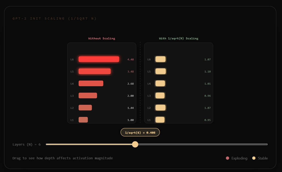
Look at what the residual connections actually do across a deep stack. Every block takes the running representation and adds its own output on top: x becomes x plus block output, then x plus the next block’s output, over and over. Addition after addition. If each block contributes roughly unit variance, then after 12 blocks the variance of that running stream has grown with the number of blocks, and the model starts training from an unnecessarily wild place. The deeper you stack, the worse it gets.

The GPT-2 fix is a small initialization trick that’s easy to skim past in the paper. You scale down the weights of the layers that write back into the residual stream, the output projections of attention and of the feed-forward network, by a factor of 1 over the square root of the number of residual layers, 1/√N, at initialization. That’s it. It shrinks each block’s initial contribution just enough that the additions accumulate to something controlled instead of something that grows with depth. In practice the factor is 1/√(2N) where N is the number of blocks, the 2 being there because each block adds to the stream twice.

It’s the kind of detail you’d never guess you needed and would spend a long time debugging if you got it wrong, because nothing errors out. The model just trains worse for no visible reason. Every piece is now built and initialized properly. Time to run the whole thing end to end.

import torch
import math

def scale_residual_weights(W, N):
    """Returns: nested list of scaled weights, rounded to 4 decimals."""
    W_t = torch.tensor(W, dtype=torch.float64)
    scale = 1.0 / math.sqrt(N)
    result = W_t * scale
    return [[round(float(v), 4) for v in row] for row in result]

def forward_with_scaling(x, weights_list, N, use_scaling):
    """Returns: L2 norm of final activation as float, rounded to 4 decimals."""
    x_t = torch.tensor(x, dtype=torch.float64)
    for W in weights_list:
        W_t = torch.tensor(W, dtype=torch.float64)
        if use_scaling:
            W_t = W_t / math.sqrt(N)
        x_t = x_t + W_t @ x_t
    return round(float(torch.norm(x_t).item()), 4)

The Full Forward Pass

This is where the pieces stop being pieces. A sequence of token IDs goes in one end and a prediction for the next token comes out the other.

The path is: look up the token embeddings, look up the position embeddings, add them together. Push that through all 12 decoder blocks in sequence, each one refining the representation a little more. Run the one final layer norm that pre-norm architectures tack on at the end. Then project the result back out to vocabulary size, producing a score for every one of the 50,257 possible next tokens, at every position in the sequence.

The one detail I’d flag here is weight tying. That final projection from 768 dimensions back to 50,257 needs a big matrix, and GPT-2 doesn’t learn a new one. It reuses the token embedding matrix you built way back at the start, just transposed. The same table that turns token IDs into vectors on the way in turns vectors back into token scores on the way out. It saves a large chunk of parameters, and there’s a clean intuition to it: the representation of a token and the thing you compare against to predict that token should live in the same space.

What comes out is a distribution over the whole vocabulary at every position. Which is a model that can score next tokens. It is not yet a model that generates anything. For that you have to actually pick tokens and feed them back in.

import torch
import torch.nn.functional as F
import math

def gpt2_forward(token_ids, wte, wpe, layers, gamma_f, beta_f, W_lm):
    token_ids_t = torch.tensor(token_ids, dtype=torch.long)
    wte_t = torch.tensor(wte, dtype=torch.float64)
    wpe_t = torch.tensor(wpe, dtype=torch.float64)
    gamma_f_t = torch.tensor(gamma_f, dtype=torch.float64)
    beta_f_t = torch.tensor(beta_f, dtype=torch.float64)
    W_lm_t = torch.tensor(W_lm, dtype=torch.float64)

    seq_len = len(token_ids)
    d_model = wte_t.shape[1]
    n_heads = 12
    d_head = d_model // n_heads

    positions = torch.arange(seq_len)
    x = wte_t[token_ids_t] + wpe_t[positions]

    mask = torch.tril(torch.ones(seq_len, seq_len, dtype=torch.float64))

    for layer in layers:
        W_q = torch.tensor(layer["W_q"], dtype=torch.float64)
        W_k = torch.tensor(layer["W_k"], dtype=torch.float64)
        W_v = torch.tensor(layer["W_v"], dtype=torch.float64)
        W_o = torch.tensor(layer["W_o"], dtype=torch.float64)

        g1 = torch.tensor(layer["gamma1"], dtype=torch.float64)
        b1 = torch.tensor(layer["beta1"], dtype=torch.float64)

        W1 = torch.tensor(layer["W1"], dtype=torch.float64)
        bias1 = torch.tensor(layer["b1"], dtype=torch.float64)
        W2 = torch.tensor(layer["W2"], dtype=torch.float64)
        bias2 = torch.tensor(layer["b2"], dtype=torch.float64)

        g2 = torch.tensor(layer["gamma2"], dtype=torch.float64)
        b2_ln = torch.tensor(layer["beta2"], dtype=torch.float64)

        ln1 = F.layer_norm(x, (d_model,), weight=g1, bias=b1, eps=1e-5)

        Q = ln1 @ W_q.T
        K = ln1 @ W_k.T
        V = ln1 @ W_v.T

        Q = Q.view(seq_len, n_heads, d_head).permute(1, 0, 2)
        K = K.view(seq_len, n_heads, d_head).permute(1, 0, 2)
        V = V.view(seq_len, n_heads, d_head).permute(1, 0, 2)

        scores = Q @ K.transpose(-2, -1) / math.sqrt(d_head)
        scores = scores.masked_fill(
            mask[:seq_len, :seq_len].unsqueeze(0) == 0,
            float("-inf")
        )

        weights = torch.softmax(scores, dim=-1)
        attn_out = weights @ V

        attn_out = attn_out.permute(1, 0, 2).reshape(seq_len, d_model)
        attn_out = attn_out @ W_o.T

        x = x + attn_out

        ln2 = F.layer_norm(x, (d_model,), weight=g2, bias=b2_ln, eps=1e-5)

        h = ln2 @ W1.T + bias1
        h = 0.5 * h * (
            1.0
            + torch.tanh(
                math.sqrt(2.0 / math.pi)
                * (h + 0.044715 * h.pow(3))
            )
        )

        h = h @ W2.T + bias2
        x = x + h

    x = F.layer_norm(
        x,
        (d_model,),
        weight=gamma_f_t,
        bias=beta_f_t,
        eps=1e-5
    )

    logits = x @ W_lm_t.T

    return logits.tolist()

Greedy Decoding

The forward pass hands you scores over the vocabulary. Generation is the loop that turns those scores into an actual sequence, one token at a time.

The simplest possible version is greedy decoding. You run the forward pass, look at the scores for the last position, take the single highest-scoring token, append it to your sequence, and feed the whole extended sequence back in to get the next one. Repeat until the model emits the end-of-text token or you hit a length limit. That’s the entire loop.

It’s the cleanest way to confirm the model works, and it has one obvious flaw once you watch it run. Because it always takes the single most likely token, it’s completely deterministic, the same prompt gives you the exact same output every time, and worse, it tends to fall into loops. It’ll latch onto a phrase and repeat it, because the most probable next token after a phrase is often the token that starts the phrase again. Greedy gets you generation. It doesn’t get you generation you’d want to read.

To fix that you need to let the model be a little less sure of itself, on purpose.

import torch

def greedy_decode(input_ids, logits_map, num_steps):
    """Returns: list of int (full generated sequence including input_ids)"""
    ids = list(input_ids)
    for _ in range(num_steps):
        key = tuple(ids)
        if key not in logits_map:
            break
        logits = torch.tensor(logits_map[key], dtype=torch.float32)
        next_token = torch.argmax(logits).item()
        ids.append(next_token)
    return ids

Top-k Sampling

The fix is to sample instead of always taking the maximum, but sample carefully, with two knobs.

The first knob is temperature. Before turning the scores into probabilities, you divide them all by a temperature value. Below one, the distribution gets sharper and the model leans toward its top picks, closer to greedy. Above one, it flattens out and the model gets more adventurous. It’s a single dial for how much risk the model takes on each token.

The second knob is top-k. Even after temperature, you don’t want the model reaching into the long tail of genuinely bad tokens, the thousands of options with tiny probabilities that are mostly noise. So you keep only the k highest-scoring tokens, throw the rest away by setting them to negative infinity, run softmax over just those survivors, and sample from that. Now the model has real choice, it can take the second or third option sometimes, which breaks the repetition loops that greedy fell into, but it can only choose from tokens that were plausible in the first place.

Between the two, you get controlled randomness. Enough variety that the output stops looping and starts reading like something, without so much that it wanders off into garbage. Temperature sets how bold, top-k sets how wide.

import torch

def apply_temperature(logits, temperature):
    """Returns: torch.Tensor of scaled logits"""
    return logits / temperature

def top_k_filter(logits, k):
    """Returns: torch.Tensor with non-top-k values set to -inf"""
    if k >= logits.shape[-1]:
        return logits.clone()
    values, _ = torch.topk(logits, k)
    threshold = values[..., -1]
    mask = logits < threshold
    filtered = logits.clone()
    filtered[mask] = float("-inf")
    return filtered

def sample_from_logits(logits, random_val):
    """Returns: int (sampled token id)"""
    probs = torch.softmax(logits, dim=-1)
    cumsum = torch.cumsum(probs, dim=-1)
    token_id = (cumsum >= random_val).long().argmax().item()
    return token_id

Conclusion

By the end, I had rebuilt the core of GPT-2 from scratch: a byte-level tokenizer, learned token and positional embeddings, masked multi-head self-attention, feed-forward blocks with pre-norm, tied embeddings, and a sampling loop that could generate text.

The generations weren’t impressive, and that was never the point. The point was to stop treating transformers like a black box. Reading the paper and watching Karpathy’s walkthrough taught me what each component does. Implementing them myself, breaking things, debugging them, and seeing the failures taught me why they exist.

Instead of tackling the entire architecture at once, I built each component as a separate problem on TensorTonic. That made the learning process much more manageable and forced me to understand every building block before moving on.

Resources

• GPT-2 Paper: Language Models are Unsupervised Multitask Learners
• TensorTonic: https://www.tensortonic.com/