Euler’s Runge-Kutta — Numerical Integration

After explaining numerical differentiation and Richardson exploration in this article series. This article illustrates numerical integration.

Image Reference: precisionformedicine.com

Numerical Integration

As we know, integrals are the area under the continuous curve. We want to estimate an area for our discrete data points when discussing numerical integration. To do so, we can use one of these two methods.

Trapezoidal rule

We connect the consecutive points and project each point on the x-axis. Hence, we obtain trapezoids next to each other. All we have to do now is to calculate the sum of all their areas.

Trapezoidal rule (Reference: pythonnumericalmethods.berkeley.edu)

The area of a trapezoid is:

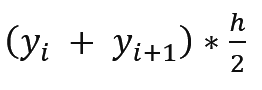
Area in our case:

Using this type of integration also means that the calculation will result in some errors, so the proper way to write this equation is:

Having this error means we can also benefit from Richardson’s approximation to have better results, so we’ll use the same rule as the one derived before:

Midpoint Rectangular Rule

We take a point that has a point before, and after making it the middle one, we draw a line parallel to the x-axis to reach the value of x of the previous point and the x of the point after. Then from the two points, before and after the point we chose, we project them on the x-axis, forming a rectangle from a midpoint.

Midpoint Rectangular rule (Reference: tutorial.math.lamar.edu)

Area of rectangle:

Since we have opposite side equal, we can use y of odd indices and multiply them by 2h

Area in our case:

The error is also found here so Richardson also applies:

The two methods we used previously (midpoint rectangular and trapezoidal) have errors due to how they obtain their shapes. The figure above shows how the shapes took either more or less area under the curve. That is why we can combine these two rules to form a method that takes the right amount of area from both rules to decrease the margin of error.

This new rule obtained is called Simpson’s Rule:

Richardson has helped to find better approximations for both numerical differentiation and integration. We almost derived the same equation each time using it except when having a larger h in central difference. Therefore, we can derive a more generalized form of Richardson, dealing with the lag as well:

As we saw in the previous table where we took [h=0.5, h=0.25, h=0.125] (article 2/4), that was because the difference of h we used to get Richardson with equation [a] and [b] was 2h. So, in general, when we use q h*, and start from lag = c, we use multiples of qc in our table.

Now with all of the numerical differentiation, Richardson extrapolation, and numerical integration being explained, we can combine this knowledge to comprehend the final piece in this series that will focus on the Runge-Kutta.