A Practical Guide for Designing Rigorous Retention Experiments
How to test multiple offers, measure true causal impact, and avoid common pitfalls
A Practical Guide for Designing Rigorous Retention Experiments
How to test multiple offers, measure true causal impact, and avoid common pitfalls
When you’re testing retention offers to reduce churn, the stakes couldn’t be higher. You need clean causal evidence — not just correlations or hopeful patterns. After working through dozens of retention experiments, I’ve learned that success comes down to marrying rigorous statistical design with operational reality.
This blog is a guide that walks you through a structured approach to designing and running multi-arm experiments with data science rigor that definitively answer: “Which retention offer actually reduces churn?”
N.B: Although this guide is for A/B/n testing, it is equally generalizable for simpler A/B testing (barring multi-comparison correction for FWER).
Start with Crystal-Clear Objectives
Before writing a single line of code or launching any campaign, nail down your goals.
You’re not just measuring renewal rates. You’re identifying the incremental causal lift each offer generates compared to doing nothing (or sending a generic reminder).
Your Primary Goal: Measure incremental lift in renewal from each offer versus a control group.
Primary Outcome: Renewal within a specified window (typically 60 days before the due date).
Business Outcome: Incremental profit per user = (incremental renewals × margin or LTV) — offer cost
Remember: an offer might boost renewals by 5 percentage points, but if it costs more than the value it creates, it’s not worth deploying.
Pre-Register Your Hypotheses (Yes, Really)
Pre-registration is your insurance against p-hacking and post-hoc storytelling. Write down exactly what you’re testing before you launch.
Let’s say you have a control group (no offer) and four test offers: A, B, C, and D.
Primary Hypotheses (One-Sided Tests vs Control):
For each offer, test whether it beats the control:
- Does Offer A increase renewal rates versus control?
- Does Offer B increase renewal rates versus control?
- (And so on for C and D)
Use Dunnett adjustment/Bonferroni correction/Šidák correction to control familywise error (FWER) across these multiple comparisons.
Secondary Questions (Exploratory): How do offers compare to each other pairwise?
Heterogeneity Analysis: Pre-specify moderators like churn risk decile, tenure, plan price, or region. These help you understand if certain offers work better for specific customer segments.
Your Decision Rule: The winner is the arm with the highest incremental profit, not just the highest renewal rate.
Define Your Target Population Precisely
Targeting “at-risk customers” isn’t specific enough. Define your frame with surgical precision.
Who’s In:
- Customers approaching renewal within your defined churn window
- Reachable through your chosen channel
Who’s Out:
- Legal or compliance restrictions
- Users who opted out
- Prior promotional exposure (avoids contamination)
- Unpaid balances
- VIPs (if policy restricts offers)
Critical Timing Move: Freeze your sample frame 24–48 hours before launch. This prevents compositional shifts during randomization.
Pick One Channel: Email, SMS, or in-app — not all three. Cross-channel contamination kills clean inference.
Design Your Randomized Controlled Trial the Right Way
Unit of Randomization: Individual customers. If accounts can spill over within households, cluster by household and adjust your sample size for the design effect.
Blocking (Stratification): Your Secret Weapon
Blocking on high-signal covariates is how you supercharge statistical power:
- Churn risk deciles or quintiles
- Macro-region
- Week (essential for multi-week tests)
Blocking ensures every treatment arm has similar distributions of key variables. This cuts variance and boosts power without creating design effect penalties.
Why Block by Week?
If your test runs across several weeks with capacity constraints, time becomes a confounder:
- Seasonality (paydays, holidays, launches)
- Marketing noise (other campaigns)
- Operational drift (send timing issues)
- Composition shifts (who becomes eligible each week)
By blocking on week, you randomize individuals separately within each week. Every arm appears in every week with equal share. Without week blocking, random chance might give one arm more “tough week” users and another more “easy week” users. Your observed differences would then partly reflect timing, not true offer effects.
Week blocking neutralizes time confounding and enforces true apples-to-apples comparisons.
Blocking vs Clustering: Know the Difference
People often confuse these terms:
Blocking: Individual randomization within strata to reduce variance. No penalty. Use by default.
Clustering: Group randomization to avoid interference. Requires sample size inflation and robust standard errors. Only use when operationally necessary.
For retention tests: Block by Week × (Risk × Region). Only cluster if you face household spillovers, agent pod constraints, or geographic phasing requirements.
Example 4-Week Setup:
- Arms: Control, A, B, C, D (5 total)
- Weekly capacity: 4,000 contacts
- Allocation: 800 per arm per week
- Randomize within each Week × Risk quintile × Region
- After 4 weeks: ~3,200 users per arm
Allocation Strategy: Equal splits work. If testing many offers, consider 2× control size for better power.
Exposure Controls: Single channel, consistent timing, one-exposure rule. No user should see multiple offers.
Build Instrumentation That Makes Analysis Trivial
Clean logging determines whether analysts (including future you) can reconstruct your experiment.
Core Tables:
- assignment: user_id, block_id, arm, rand_seed, assigned_ts
- exposure: user_id, arm, send_ts, delivered, opened, clicked (diagnostic only)
- outcome: user_id, renewed_by_day30, renewal_ts, amount
- covariates: risk_score, tenure, plan, price, prior_engagement
- costs: arm, unit_offer_cost
- logs: Include trace IDs and experiment IDs everywhere
This structure makes joins trivial, balance checks easy, and sensitivity analyses straightforward.
Calculate Statistical Power (Don’t Skip This)
For binary outcomes with multiple arms, calculate sample size based on your minimum detectable effect (MDE).
Use Dunnett adjustment (preferred) or Bonferroni correction or Šidák correction for multiple comparisons against shared control.
Example (60% Baseline Renewal Rate):
- Detect +3pp lift at 80% power, one-sided α = 0.01 → ~5,300 per arm
- Detect +2pp lift → ~11,900 per arm
- Detect +5pp lift → ~1,900 per arm
Power Boosters:
- Stratify on strong predictors
- Use covariate adjustment (CUPED) with pre-period data — often cuts variance 10–30%
- Increase control group size
Pre-Specify Your Analysis Plan
Write your exact analysis approach before seeing data. This prevents the temptation to slice until you find significance.
Primary Analysis: Intention-to-treat (ITT) risk difference for each offer vs control.
Use Dunnett or any other applicable (like Bonferroni/Sidak etc.) adjustment for familywise error control. Report 95% confidence intervals and adjusted p-values.
Regression Model:
logit(renewed) ~ arm + risk_decile + week + region + [pre-period covariate]
This adjusts for stratification and applies CUPED for precision.
Analysis Checklist:
- Check randomization balance
- Compute ITT effects (by assignment, not exposure)
- Apply Dunnett or Holm adjustment
- Report confidence intervals, not just p-values
- Calculate incremental profit per arm
Control for Bias and Validate Assumptions
SUTVA (No Interference): Prevent cross-exposure between arms. Cluster by household if spillover is likely.
Stable Exposure: Same timing and channel across arms.
No Selective Attrition: Track reachability equally. Investigate if delivery rates differ.
No Peeking: Pre-commit to sample size or use formal sequential methods.
Fairness: Monitor effects across protected classes. Review high-value discounts for risk.
Pre-Commit to Your Decision Rule
If offers beat control (after adjustment): Choose the one with highest incremental profit.
If nothing beats control: Don’t launch. Revisit creative or targeting.
The Dry-Run Isn’t Optional
A dry-run isn’t statistically required, but operationally it’s mandatory. Think of it as insurance against disasters: botched randomization, broken logging, missed suppressions, capacity blowups.
Goal: Verify the experiment’s plumbing and governance — not estimate lift.
What You Need: A signed green sheet confirming:
- Definitions locked
- Randomization reproducible
- Quotas correct
- Events flowing to logs
- Capacity safe
Treat the dry-run as a go/no-go gate before Week 1.
Parallel vs Sequential Testing: Strategic Tradeoffs
Parallel A/B/n (Recommended)
Run Control + all offers simultaneously in the same time window.
Pros:
- Time effects cancel (same period)
- Best sample efficiency (shared control)
- Fastest decision
Cons:
- Operationally heavier (more creatives live)
Sequential Testing (One Offer at a Time)
Sometimes operational constraints force sequential testing.
What Changes:
- Time becomes a confounder: Seasonality, competition, and fatigue vary across periods
- No shared control: Re-estimate control each period (larger sample, longer time)
- Inference needs time fixed effects: Use CUPED and robust SEs
When Sequential Works:
- Call center can only handle one offer
- Legal gates each creative individually
- Rapid creative iteration
Key Risks:
Temporal Drift: Differences could reflect time, not offers
Carryover Effects: Offer A exposure changes responses to Offer B
Population Depletion: Early periods get easy wins; later periods face tougher users
Multiple Testing: Repeated looks inflate Type-I error
Winner’s Curse: Observed winners have inflated effects
Mitigation for Sequential:
Use regression with time FE: logit(renewed) ~ arm + week + risk_decile + region + [CUPED covariate]
- Cluster SEs by time block
- Add CUPED with pre-period propensity
- Report effects vs persistent control
- Provide sensitivity excluding volatile weeks
Consider maintaining a persistent control stream across all periods for better comparability.
The Bottom Line
Rigorous retention experiments aren’t just statistical exercises. They’re about marrying causal inference with operational constraints.
By pre-registering hypotheses, blocking smartly, running clean ITT analyses, and pre-committing to decision rules, you build experiments people trust — and you make better business decisions.
This framework scales whether you’re testing two offers or ten, running for two weeks or two months. Adapt the details to your context, but hold firm on the core principles: causality, reproducibility, and business clarity.
Now go design an experiment that ships real results.
What’s been your biggest challenge running retention experiments? Drop a comment — I’d love to hear your war stories and lessons learned.
P.S.: In my experience, most of the organizations starting out on the causal experiment design journey struggle with understanding and calculation of statistical power/sample size/MDE.
In the next post, I use a simple Python script to create a table or grid for Statistical Power/Sample size/MDE calculation for reference. Stay tuned!….
메타데이터
- post_id
- 57a9c2fa8b2b
- slug
- designing-rigorous-retention-experiments-a-practical-guide-for-marketing-technical-teams-57a9c2fa8b2b
- url
- https://medium.com/@elkayvee/designing-rigorous-retention-experiments-a-practical-guide-for-marketing-technical-teams-57a9c2fa8b2b
- canonical_url
- https://medium.com/@elkayvee/designing-rigorous-retention-experiments-a-practical-guide-for-marketing-technical-teams-57a9c2fa8b2b
- author_url
- https://medium.com/@elkayvee
- status
- ok
- fetched_at
- 2026-06-09 15:37:30