Testing hypotheses about proportions (%) through the logistic regression (and friends) — part I

In my previous article titled “Is logistic regression a regression? It has been a regression since its birth — and is used this way every day.” I explained why the common misconception that “logistic regression is not a regression” is fundamentally flawed on the statistical ground. I also showed numerous fully regression-related applications of the logistic regression that are daily used in my field — clinical trials.

This time, I want to focus more on the model- based testing (I made a few notes on GitHub, alas — lacking time to continue…), where the logistic regression just shines, allowing one not only to replicate a variety of the classic statistical tests of proportions (%), but also to extend them by allowing one to:

• account for multiple grouping factors; handling multiple categorical predictors, which levels form groups across which we can compare proportions (%), enables the n-way ANOVA-like analyses. Actually, for the non-Gaussian members of the Generalized Linear Model family the term “analysis of variance” becomes “analysis of deviance”. Testing can be done via Wald’s, Likelihood Ratio and Rao score framework
• adjust the testing for numerical covariates (just like in ANCOVA)
• include interactions between all types of predictors
• employ the exact parametric “MVT” adjustment for multiple comparisons (based on the multivariate t distribution; yes, the same that if combined with appropriate contrasts, results in the Tukey’s HSD all-pairwise and Dunnett’s all-vs-baseline tests)
• test for trends in proportions (%) over time
• handle repeated observations (e.g. paired) if the GEE (Generalized Estimating Equations) estimation is employed

…and more.

Isn’t it just awesome addition to just the classic 2-sample z test for proportion or chi2 test of multiple proportions?

Let’s briefly see what tests can be replicated (links refer to my GitHub examples) through the ordinary logistic regression and a few “friends”: ordinal logistic regression, conditional logistic regression and GEE-estimated logistic regression:

1. the Wald’s (normal approximation) **z test for 2 proportions with non-pooled standard errors* (common in clinical trials). Testing is done via EM-means (estimated-marginal means) on the probability scale or the AME (average marginal effect*) over the binary predictor distinguishing the two compared groups.
2. the Rao’s score (normal appr.) **z test for 2 proportions with pooled standard errors** (just what the prop.test() does in R)
3. the chi2 test for multiple (2+) proportions
4. ANOVA-like (joint) test for multiple caterogical predictors (n-way ANOVA). Also (n-way) ANCOVA if you employ numerical covariates.
5. the **Cochran-Mantel-Haenszel (CMH) for stratified/matched data* via conditional logistic regression*
6. the **Breslow-Day test for odds ratios** through Rao’s ANOVA → the interaction term
7. the **Cochran-Armitage test for trend in ordered proportions**
8. the McNemar and Cochran Q test of paired proportions via GEE estimation (Generalized Estimating Equations with compound symmetry)
9. the **Friedman test** — as above
10. the **Mann-Whitney-Wilcoxon and Kruskal-Wallis** via Ordinal Logistic Regression (and paired Wilcoxon via GEE)

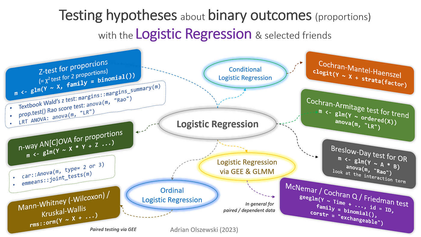
Showing the direct relationships for all listed tests would be rather challenging and make this article extremely long.

So let’s pick something really cool (at least to me 😉) — let’s prove, that the equivalence between the 2-sample Wald’s z-statistic for comparing proportions with unpooled variances and the Average Marginal Effect over logistic regression with a single binary predictor.

—

⚠️Disclaimer: What you will read below demonstrates the algebraic equivalence between selected classical hypothesis tests and their model-based analogues under common large-sample assumptions. My goal was to show how the formulas transition from one framework to another. The derivations focus on analytic equivalence of test statistics and do not provide a fully rigorous proof of asymptotic distributions or verify all regularity conditions required in formal statistical theory. As such, this note should be viewed as a proof of concept and kind of a “conceptual bridge” rather than a complete theoretical course. In particular: distributional assumptions are stated informally rather than derived formally, asymptotic arguments (e.g., convergence to χ² distributions) are not proven (it is not a textbook!), conditions required for likelihood-based theory are not verified.

So, if you prepare for an exam, use it with care.

—

We will assume independent binomial sampling and no small-sample corrections. The Wald’s z-statistic for difference in 2 proportions with unpooled variances is of the following form:

Where p1 stands for the estimated probability (sample proportion, %) in the 1st group, p2 is the estimated probability (sample proportion, %) in the 2nd group, n1 and n2 denote respective group sizes. I will show that this statistic is 1:1 equivalent to the average marginal effect (AME) of the logistic regression with a single binary predictor playing role of indicator for the compared samples.

To simplify calculations, I will show the equivalence of the nominator and denominator of the z statistic, i.e. the difference between two probabilities and its variance, separately.

The equation of logistic regression

Let’s start from the equation of the logistic regression with a single binary predictor:

or equivalently, after applying the inverse-logit, i.e. sigmoid function (let’s also simplify X1 to X)

(Average) Marginal Effect

Now, let’s introduce the marginal effect (ME) of a regression model. The ME of a given predictor variable X is the slope of the regression surface with respect to X, reflecting the rate at which Y changes at a given point with respect to X, while holding values of all other predictors constant. In other words, ME is an instantaneous rate of change, calculated as partial derivative of the regression equation with respect to X. For example, for an equation: Y = β0 + β1X1+ β2X2 + β3X1X2 corresponding ME(Y, X2) = ∂Y/ ∂X2 = β2 + β3*X1.

The average marginal effect (AME) calculates ME at every observed value of X and averages across the resulting effect estimates. In other words, AME is an average effect of an infinitesimal change in X across all observations:

For a generally defined equation:

the partial derivative (using the quotient rule and rewriting back in terms of σ) is of the form:

Therefore,

AME for the binary predictor

For a categorical predictor, however, there is no something like “infinitesimal change”. There is just switch between categories, so the AME becomes a contrast, i.e. a difference between values of the appropriate partial derivative calculated at the selected category levels, thus:

Which means, that the AME for such defined logistic regression corresponds to a difference in two estimated group probabilities, expressed in percentage points.

Variance of AME for the binary predictor

Now, I will show the equivalence between the variance in the Wald’s z statistic and the variance of the AME for the binary predictor.

Several replacements will save a lot of typing:

• P A = p ( Y = 1 | X = A ) , P B = p ( Y = 1 | X = B )
• P i × ( 1 − P i ) = P i Q i

Let’s introduce the AME function:

Let’s also encode the two levels {A, B} using a single binary predictor X such that: A: X=0, B: X=1, let’s express PA and PB in terms of beta coefficients:

so the AME function is now expressed as:

The variance for the AME is typically obtained by the delta method:

Let’s first obtain the derivatives. Recall, that:

Therefore,

Now, we need the variance-covariance matrix, i.e.

This can be obtained by inverting the Fisher information matrix given by:

where X is the design matrix with 2 columns ( β0 of ones and β1 indicating when X=1), with nA and nB number of rows corresponding to group A and B, respectively.

and W is the diagonal matrix of weights, of the block-diagonal form:

which can be simplified to:

where InA and I B are respective identity matrices.

The multiplication result can be abbreviated to appropriate sums:

where 1 is the result of multiplying 1 x 1 (the β 0 vector), and Xs refer to the other products of the β 0 and β 1 vectors. Since these vectors consist only of 0 and 1, and 0 refers to the “A” group and 1 refers to the “B” group, their products keep only the “B” part. Therefore, the final result is:

So the inverse can be computed (remembering that both covariance elements are equal):

After simplifying the denominator term:

finally:

By recalling formula #13 and matrix #15, we can express the variance of AME as:

which expands to:

Let’s replace P∗Q , the variance, with V to simplify (note: I occasionally use “×” to denote arithmetic multiplication to facilitate reading; A×B is just AB):

Therefore,

This way I have shown the equivalence of the 2-sample Wald’s z-statistic for comparing proportions with unpooled variances and the average marginal effect of the logistic regression with a single binary predictor distinguishing the compared samples.

Also, since the Estimated Marginal Means (EM-Means) on so defined logistic regression and “re-grided” to the probability scale represent the estimated probabilities, the contrast comparing them through the Wald’s approach yields exactly the same result. Although some minor discrepancies exist due to Maximum Likelihood Estimation, even for so small samples (N=10 and 20) the agreement is just perfect.

Average Marginal Effect

> wald_z_test_non_pooled(x1 = 6, n1 = 20, x2 = 10, n2 = 20)
  diff         z    chi2        se  p.value  p.value_1        LCI        HCI
1 -0.2 -1.318761 1.73913 0.1516575 0.187249 0.09362452 -0.4972433 0.09724326
> 
> data <- data.frame(response = factor(c(rep("Success", 6), rep("Failure", 20-6),
+                                        rep("Success", 10), rep("Failure", 20-10))),
+                    grp    = factor(rep(c("B", "A"), each=20)))
> 
> m <- glm(response ~ grp, data = data, family = binomial(link = "logit"))
> data.frame(marginaleffects::avg_slopes(m)) %>% mutate(across(where(is.numeric), ~round(., 6)))
  term contrast estimate std.error statistic  p.value  s.value  conf.low conf.high
1  grp    B - A     -0.2  0.151657 -1.318762 0.187249 2.416973 -0.497243  0.097243

EM-means

> library(emmeans)
> update(pairs(emmeans(m, specs = ~grp, regrid="response")), infer = c(TRUE, TRUE)) %>% 
+     data.frame() %>% 
+     mutate(across(where(is.numeric), ~round(., 6)))
  contrast estimate       SE  df asymp.LCL asymp.UCL  z.ratio  p.value
1    A - B      0.2 0.151657 Inf -0.097243  0.497243 1.318761 0.187249

I used this implementation of the z statistic with unpooled variances:

wald_z_test_non_pooled <- function(x1, n1, x2, n2, conf.level=0.95) {
    p1 <- x1/n1
    p2 <- x2/n2

    se_p1 <- sqrt(p1 * (1 - p1) / n1)
    se_p2 <- sqrt(p2 * (1 - p2) / n2)

    se_diff <- sqrt(se_p1^2 + se_p2^2)

    z <- (p1 - p2) / se_diff
    p <- 2 * (1 - pnorm(abs(z)))
    hCI <- abs(qnorm((1 - conf.level)/2)) * se_diff
    return(data.frame(diff=p1-p2,
                      z = z, chi2 = z^2,
                      se = se_diff, 
                      p.value = p, p.value_1 =p/2,
                      LCI = (p1-p2) - hCI,
                      HCI = (p1-p2) + hCI,
                      row.names = NULL))
}

If these formulas render badly on your screen, you can find it also on my GitHub: https://github.com/adrianolszewski/Logistic-regression-is-regression/blob/main/logistic_regression_AME_Wald_z_test_proportions.md

In the next articles I will try to prove other relationships, so stay tuned!

Visit:

1. Testing hypotheses about proportions (%) through the logistic regression (and friends) — part II