A Newtonian Secret Hiding in Einstein’s Gravity

A Euclidean Approach to the Schwarzschild Metric

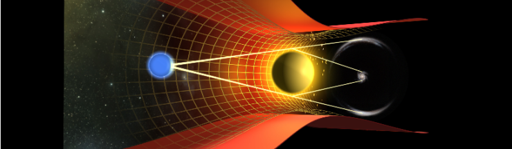
NASA/ESA Hubble image (public domain). Source: Wikimedia Commons

Shortly after Einstein published general relativity in 1915, the British astronomer Arthur Eddington — who would later confirm the theory by measuring the bending of starlight — was asked whether it was true that only three people in the world understood the theory. Eddington paused. His colleague suggested he was being modest. Eddington replied, “On the contrary — I’m trying to think who the third person is.” (1)

If general relativity feels difficult, you are in good company. Even many physicists find its mathematics forbidding. I’m certainly no specialist myself, though I’ve attended my share of GR lectures. What I can do — and what this article tries to show — is that one of GR’s central results contains a clue that Newton left in plain sight.

In particular, we will see how the temporal part of the Schwarzschild solution — the piece that describes gravitational time dilation — can be reconstructed from Newton’s law, a few interpretive assumptions, and basic math. No curvature, no tensors, no Einstein field equation. Just Newton’s gravity, understood in a slightly different way.

This article is part of a broader effort to rebuild an intuitive, pictorial understanding of physics. I have found that this approach both aids understanding and, frankly, inspires me to keep learning. I hope it proves useful to you as well.

Most GR Math Looks Impossible — the One Equation That Isn’t

The mathematics of general relativity is formidable. Working with the full Einstein field equations requires fluency in tensor calculus, index notation, covariant derivatives, Christoffel symbols, and much more.

But there is one part of GR where the physics becomes beautifully simple. First, assume a perfectly spherical mass and look only at the empty space around it. Derive the math. In 1915, Karl Schwarzschild discovered that the equations simplify dramatically — while serving on the Russian front in World War I, no less — and produced the first exact solution to Einstein’s field equations. Einstein was astonished. He wrote back, “I did not expect that one could formulate the exact solution of the problem in such a simple way.” (2)

Simple? Really?

For Einstein, maybe. For me, not so much. I include the complete form in an addendum at the end of this article, along with more discussion. But what we will use, and all that we will need, is the temporal part of Schwarzschild’s solution:

Equation 1:

In this expression, dτ is the increment of proper time — the time measured by a clock located at radius r. This temporal part of the Schwarzschild metric tells us exactly how that clock runs relative to coordinate time t. The constants G, M, and c are the gravitational constant, the mass of the central object, and the speed of light, while r is the radial distance from the center of that mass.

Schwarzschild’s original derivation is a masterpiece of mathematical physics. The equations were intricate and extensive, employing the full apparatus of general relativity. His method was rigorous, elegant, and historically important — but it is not simple.

We are not going to follow his path.

This article attempts something different: a new interpretation of the foundations and assumptions underlying the Schwarzschild result, built from Euclidean geometry, a Newtonian context, and a fresh understanding of its temporal term. Rather than deriving the metric from the Einstein field equations, we will reconstruct its meaning using simpler terms and assumptions.

Basic Assumptions for Readers New to This Approach

This article builds on two earlier articles published in Medium — one on gravity and one offering an alternative interpretation of special relativity. It is not necessary to read those to follow what comes next. What follows are just the minimum necessary assumptions drawn from those earlier works.

In the relativity article, I introduced a simple analytic model in which physical objects are represented as line‑objects composed of discrete cels, as illustrated in the following diagram. Each cel moves at velocity c in an abstract structurocausal space. In this setting, the vector c can be rotated in structurocausal space. Its vertical component becomes c/γ, corresponding to the apparent passage of time, while its horizontal component becomes the causal/spatial velocity v.

In the diagram, line‑object A moves vertically downward to and through the causal axis (which stands in for the x, y, and z axes), while line‑object B approaches at an angle θ relative to the vertical. To make these relationships more obvious, I include a side-rendering of the vector c for a cel in object B.

Diagram 1

When a cel intersects the causal axis, it generates an event (hence the name “causal” axis), so the apparent progression of time — but not time itself — is determined by the rate at which cels reach that axis. A line‑object moving vertically through the causal axis produces events at the maximal rate. A line‑object whose c‑vector is rotated into the spatial direction produces events more slowly, by a factor 1/γ relative to the vertical case. This generates the Lorentz factor in the model, and the proper‑time equation

Equation 2:

dτ² = (1 − v²∕c²) dt²

is already built into the structurocausal model.

The relativity article cited earlier shows that these events can be unambiguously mapped from structurocausal space onto a standard Minkowski spacetime diagram, fully consistent with special relativity. No new mathematics is introduced using this approach. The structurocausal model and the mapping simply provide a different underlying framework for understanding the same physics.

A note for the technically inclined. This approach may appear to smuggle in an absolute, almost Newtonian framework. In a limited sense, it does: the structurocausal model treats the event‑rate of a line‑object as an objective quantity, and a rotated c‑vector genuinely produces a slower rate of event‑generation, which appears as slowed temporal progression. But this “absolute” structure applies only to the underlying Euclidean framework. The relativity article shows how this base structure translates cleanly and without contradiction into the full set of relativistic relationships uncovered by Einstein. Readers interested in that deeper foundation can find the complete argument there; for present purposes, only the minimal assumptions summarized above are required.

Velocity and the addition of velocity in this model

In this article, a new interpretation of velocity addition is required and follows directly from our base assumptions. Velocity in this model arises from the rotation of a cel’s c‑vector, as suggested in Diagram 1. Because of this, velocity vectors cannot “add” in the conventional sense, or even in Einstein’s original sense, since the maximum speed is already constrained. Nonetheless, Einstein’s velocity‑addition rule emerges naturally within the model and was demonstrated in the cited paper on relativity.

For further intuition, note that a line‑object’s velocity is not an independent quantity that can be added to another. Velocities in a moving frame do not exist sui generis; they are simply rotated components of c. We cannot take an object moving at 0.7 c in a frame taken to be 0.8 c and treat that 0.7 c component as having some independently valid existence. A velocity is only a rotated component of the underlying c‑vector, and the component “0.7 c” does not exist inside a frame moving at 0.8 c. This viewpoint may seem unusual, but it simplifies the kinematics and makes them more intuitive. Once the rotated c‑vector is expressed in both frames, the familiar velocity‑addition expression follows directly from relating those components.

This interpretation of velocity — as a rotated component of c rather than an independent quantity — allows the velocity‑addition rule to be derived entirely within Euclidean geometry and (somewhat modified) Newtonian assumptions. Again, please see the relativity article if further explanation is required.

With that in place, we can now use the same idea to build our model of gravity, beginning with Newton.

A Euclidean–Newtonian Reconstruction of Gravity

In this section, we begin a Newtonian reconstruction of gravity. This is not Newton’s gravity in full, but it leans heavily on the concepts and mathematics he developed. Our first step is the construction of a velocity‑vector field, shown in the accompanying diagram. The depiction is intentionally crude and exaggerated, it is only for clarification of the concepts. The gravitational vectors v(g)) increase gradually from left to right as they approach a mass M, which in structurocausal geometry is represented as a 4‑D cylindrical hypersurface. In the diagram, we again see the line‑object B, carrying its own intrinsic velocity vector v(b).

Diagram 2:

I like to think of this process in terms of a computer analogy. The processor represents the causal axis. It takes as inputs the gravitational update v(g) and the line‑object’s vector c, with its v(b) component, and updates the system each processing cycle — let’s say every second. Think of a gravitational update of 9.8 m/s: the processor applies this update once per cycle, producing the familiar 9.8 m/s² acceleration of terrestrial gravity. The velocity field, together with Newton’s update rule, naturally leads to the differential relation dv/dt, which we will develop in the next step.

With the velocity field in place, we can now connect it to the familiar Newtonian description of gravity. Newton supplied the essential mathematics even though the modern field interpretation was developed only later.

We begin with Newton’s gravitational law:

F = GMm / r².

Newton’s second law is

F = m a.

In Newtonian terms, the gravitational field is defined as force per unit mass:

g ≡ F / m.

Substituting Newton’s gravitational law into this definition,

g(r) = (1 / m) · (GMm / r²)

Simplifying, we get:

Equation 3:

g(r) = GM / r².

Note that m does not appear in this equation. It is not needed for the update, and in fact never was. The quantity g(r) does not depend on the mass of the object being accelerated. Newton’s formulation places the test mass into the force law only to divide it back out again later. In our velocity‑field picture, the test mass is excluded at the outset: the velocity field v is the update itself, and what we usually call the “gravitational field” is just our update procedure operating on that velocity field. This means that every physical object — as represented by its line‑object — is subject to the same radial update procedure g(r) at a given radius.

The following expression captures the essential relationships:

Equation 4:

g(r) = a = dv/dt

This needs emphasis: the gravitational field is not properly a force divided by a mass. It is simply acceleration. It is simply acceleration. In other words, it is the field velocity vector with its updates, and nothing more.

Starting back toward Schwartzschild:

General relativity is written in terms of smooth differentiables operating on a manifold. So far, our model is discrete, not differentiable. But if we imagine that our update steps happen in ever smaller increments of time, the process becomes smooth. At the limit, we do indeed obtain a continuously differentiable manifold, and we can describe our velocity addition steps using differentials. And so from equations 3 and 4 we can write

dv/dt = −GM / r².

The next step is that we need to describe velocity as a function of the radius of our test mass from source mass. We need velocity as a function of radius, v(r). To get v(r), we apply the chain rule.

dv/dt = (dv/dr) × (dr/dt).

But:

dr/dt = v,

So:

dv/dt = (dv/dr) × v.

Now set this equal to the Newtonian acceleration in equation three:

Equation 5:

v (dv/dr) = −GM / r².

This is the differential equation relating velocity to radius. At this point, the variables have been separated: the velocity terms appear only on the left side of the equation, and the radius terms appear only on the right. The next step is to integrate both sides.

In order to set the bounds of integration for the leftside of equation 5, we imagine a falling object begins infinitely far from the mass, where gravity is negligible. At that location its velocity is zero:

v(∞)=0.

By the time it reaches radius r, its velocity has increased to some value we call v(r), which is the upper bound of the left‑hand integral.

For the right integral, the object travels from its starting radius ∞ to the radius r. These limits capture the cumulative gravitational influence from infinitely far away to the point of interest at radius r.

To solve Equation 5, we now integrate both sides using these bounds, as shown in the following:

Now multiply through by 2:

Equation 6: v(r)² = 2GM/r

This is the squared magnitude of the velocity field. Savvy readers will recognize the expression v(r)² = 2GM/r as the squared version of the Newtonian escape‑velocity formula. That is exactly what we should expect: escape velocity is the speed an object acquires when it falls freely from infinity to radius r, accumulating the full gravitational influence along the way — precisely the process we followed in our derivation above.

In the next step, we write out the proper‑time relation (Equation 2) with its terms squared as before.

dτ² = (1 − v(r)² / c²) dt²

Substitute in 2GM/r for v(r)² from equation 4. We obtain:

dτ² = (1 − 2GM / (c² r)) dt²

Now compare this with Equation 1 at the beginning of the article! This just is the Schwarzschild temporal coefficient. We have produced it using only Newtonian gravity and a velocity‑update field. No curvature, no tensors, no Einstein field equation.

That was easy, was it not? Then why didn’t it occur to Schwarzschild and Einstein?

The reason is that they labored (and labored very well indeed) under a misconception. In Einstein’s era, velocity was understood solely as an object’s rate of change of position in time. The idea that a fixed‑magnitude vector c could underlie motion, with the Lorentz factor emerging from Euclidean kinematics applied to that vector, simply was not available. Without that conceptual lens, the temporal Schwarzschild term could not be recognized as a kinematic consequence — a result that follows directly from Newtonian reasoning once the correct geometric framework is in place.

Conclusions

We have used a modest amount of mathematics and ignored a great deal more, yet the intuition we have reached is solid. The temporal structure of Schwarzschild’s solution — the first solution to Einstein’s field equation — was already sitting inside Newton’s gravity, waiting to be uncovered with Euclidean geometry, simple algebra, and a touch of calculus. That is an unexpectedly direct and deeply satisfying way to understand the matter. In the end, we simply found a clue for Einstein hiding in Newton’s gravity. There it was — all along.

ADDENDUM — a little more on the Schwarzschild formula:

We begin here with Schwarzschild’s 1916 full metric, of which we discussed only the temporal coefficient in the main text:

ds² = (1 − 2GM / rc²) c² dt² − (1 − 2GM / c²r)⁻¹ dr² − r² dθ² − r² sin²θ dφ².

This line element is the solution of Einstein’s field equation for a static, spherically symmetric vacuum.

Gᵤᵥ = (8πG / c⁴) Tᵤᵥ.

Under these conditions, where Tᵤᵥ = 0, the field equation reduces to Gᵤᵥ = 0.

In our derivation above, we considered the case only for a fixed radial position. In this case the spatial differentials vanish and the metric reduces to

ds² = (1 − 2GM / c²r) c² dt²,

with ds² = c² dτ² for timelike worldlines.

We now seek the last three coefficients, which are the spatial components. Two of them are trivial. The angular terms r² dθ² and r² sin²θ dφ² are simply the standard spherical‑coordinate expressions for angular displacement. Because our analysis concerns purely radial motion, the angular differentials dθ and dφ are zero for such displacements, leaving only the temporal and radial components.

To address the radial component, we are going to perform some rather simplistic math. Let us set up the following function corresponding to the radial coefficient:

f(r) = 1 − 2GM / c²r.

From the Schwarzschild temporal term, we have

dτ = √f(r) dt.

As the proper‑time factor dτ = √f(r) dt slows with radius, the corresponding radial interval must adjust in a reciprocal way so that radial light rays still satisfy ds² = 0. This requirement forces the radial coefficient to be f(r)⁻¹, exactly as in the Schwarzschild metric. The Schwarzschild metric encodes this directly:

ds²ᵣ = −f(r)⁻¹ dr².

Substituting back for f(r) gives

ds²ᵣ = −(1 − 2GM / c²r)⁻¹ dr².

This is exactly the Schwarzschild radial coefficient, obtained directly from our definition of f(r) and its role in the temporal behavior of clocks. Thus, both non‑trivial components of the Schwarzschild vacuum metric — the temporal and the radial — emerge cleanly from our velocity‑vector field construction.

And that concludes our little addendum.

Oh, and by the way, here is the title character Schwarzschild himself!

Karl Schwarzschild (public domain). Source: Wikimedia Commons

Citations

1. University of Toledo, Physics & Astronomy. “Lord Eddington.” https://astro1.panet.utoledo.edu/~ljc/lordedding.htm. Accessed July 2026.

2. Nightbase. Karl Schwarzschild (1873–1916) — German Astronomer Biography. Accessed July 2026. https://nightbase.app/FamousAstronomers/karl-schwarzschild