I Built an LLM Inference Engine on a 15 year old GPU and the Math was the Easy Part

There’s a fun lie that gets talked about AI engineering, that the hard part is the machine learning. The math. The architecture. The loss curves.

It isn’t. The hard part is making it fast. And fast is a systems problem.

I spent a few weeks building an LLM inference engine from scratch, no PyTorch, no llama.cpp, no cuBLAS. Just good old C++, a bit of CUDA, an i3–7100 running at 3.9GHz, and a GTX 750 Ti with 2GB of VRAM. What I ended up learning had almost nothing to do with transformers. It had everything to do with memory, cache lines, and why your GPU is doing a lot of nothing most of the time.

Before we get into any of that, here’s the entire operation surface of the engine, every mathematical primitive the transformer calls:

{
    matmul,
    add,
    mul,
    rms_norm,
    silu,
    rope,
    scale,
    dot,
    softmax,
    argmax
}

That’s it. Ten functions.

A 1.1 billion parameter language model, in its entirety. The intelligence is in the weights, hundreds of megabytes of learned numbers nobody fully understands. The operations are textbook. The interesting work is making it fast enough that users don’t end up doomscrolling Instagram between requests (and let’s be honest, we’ve all done it).

What You Should Know Going In

This isn’t an intro to transformers. I’ll assume you know roughly what a decoder-only LLM is: a stack of layers, each with an attention block and an MLP, that takes in a token sequence and predicts the next token.

If you want a solid primer, Andrej Karpathy’s Let’s build GPT is the best one out there.

The rest you’ll pick up as we go.

First, You Need to Open the Model

Before any math happens, you need to get the weights off disk and into memory. And how you do that is dictated entirely by how the model’s laid out on disk in the first place.

There are many formats a model can ship in, safetensors, AWQ, GPTQ, GGUF, and others. Each with its own trade-offs around quantization, tooling, and how the bytes are arranged. Throughout this project we work with a GGUF TinyLlama 1.1B model.

GGUF format, a binary file format created by Georgi Gerganov for the llama.cpp project. To understand why it’s designed the way it is, it helps to look at what’s actually inside one.

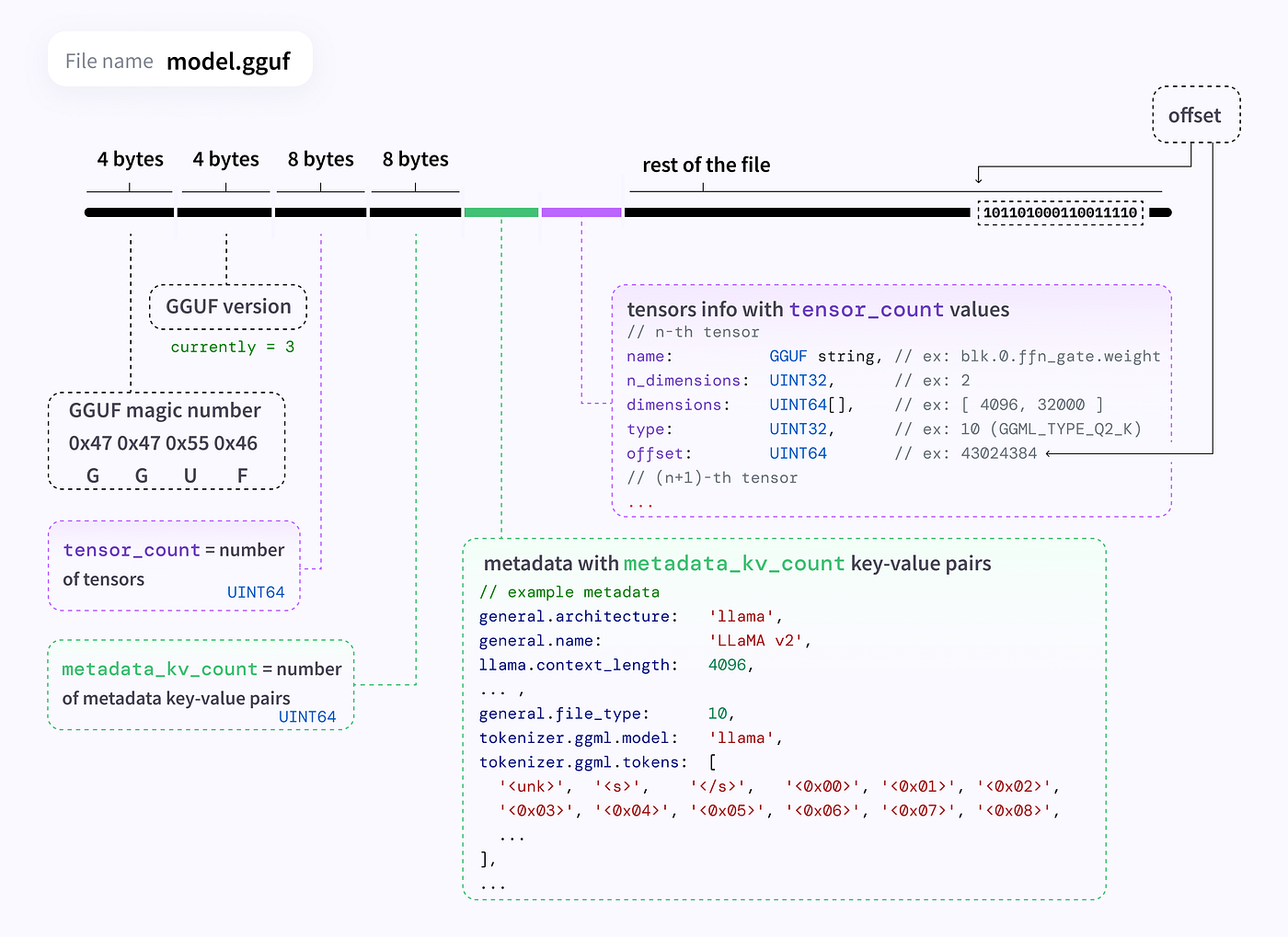
A GGUF file has three regions, laid out sequentially on disk:

The Official GGUF Specification can be found here

The file header is just a sanity check: a 4-byte magic number GGUF and a version number. If those don't match what you expect, you throw exception.

The key/value metadata section (marked as green) is where the model’s metadata lives. Every hyperparameter the engine needs is stored here as a named key: llama.context_length tells you the context length (4096 for TinyLlama 1.1B), tokenizer.ggml.model gives you the name of the tokenizer used, llama.block_count gives you the number of layers (22). You read these once at startup and use them to construct the model.

The tensor metadata section (marked as purple) is a table, one entry per weight matrix in the model. Each entry gives us metadata about each tensor parameter weight: here is a tensor named blk.0.ffn_gate.weight, it has shape [4096, 32000], it's stored in Q2_K format, and its raw bytes start at byte offset X in the file.

The raw tensor data at the bottom is just packed bytes. No framing, no separators. The offsets from the metadata table are the only way to find where one tensor ends and the next begins.

Why this format over something like HDF5 or Parquet? The key reason is that GGUF is designed to be mmap-ed. Instead of reading 700MB into RAM with read(), you call mmap() and the OS maps the file into your virtual address space. The tensor data is never actually copied, the OS pages it in from disk on demand, and the kernel's page cache handles everything. Each weight matrix is just a pointer into that mapping.

Tensor

Once the file is parsed, every weight becomes a tensor, a lightweight struct that describes where data lives and how it's shaped:

struct tensor {
    // pointer into the mmap-ed file (or GPU memory later)
    float* data;   
    uint32_t n_dimensions;

    // shape: e.g. {2048,2048} for a square weight
    vector<uint64_t> dimensions;  
    // how many elements to skip per step in each dim
    vector<uint64_t> strides;     
};

The dimensions field is the shape you’d recognize from NumPy: a 2048×2048 matrix has dimensions = {2048,2048}.

The strides field records how far apart consecutive elements sit in memory along each axis, a recipe for turning a logical (row, col) position into a flat array index. The payoff is that operations like transposes, slices, and broadcasts become free: instead of copying and reshuffling the data, you change the strides and the same underlying bytes get reinterpreted in a new layout.

At startup, the engine walks that tensor metadata table and, for each entry, builds one of these tensor structs: it reads the shape and dtype from the metadata and points data at the entry’s byte offset inside the mmap region. Each struct is then wired into the model by name, blk.0.attn_q.weight becomes layer 0’s query projection, blk.0.attn_k.weight its key projection, and so on for all 22 layers. By the time model construction finishes, every layer holds its Q, K, V, and output projection weights, but nothing has been copied. They’re all just pointers into the memory-mapped file.

Nothing loads until you touch it

The first time you actually touch a weight during a forward pass, the OS fetches the relevant page from disk — page fault. This isn’t an error, it’s the normal demand-paging mechanism. The OS loads the 4KB page containing that data, maps it into your process, and resumes execution. After that, the page lives in the kernel’s page cache and future accesses are fast.

You can see this happen directly. Running perf stat on the baseline forward pass reports over 1 million page faults at roughly 44,000 per second. That's the OS spending a non-trivial portion of inference just pulling weight pages off disk on demand.

The model is not a data structure you load. It’s a description of how to interpret a region of memory that the OS manages for you.

Two Numbers That Tell the Whole Story

Before looking at a single optimization, you need to internalize two concepts that frame everything else. They also explain the two metrics we’ll be tracking throughout.

TTFT (Time to First Token) is how long it takes to process the input prompt and produce the very first output token. During this phase, called the prefill, you’re running the full forward pass over all input tokens at once. It’s compute-heavy.

Decode latency (ms per token) is how long each subsequent token takes. During decode, you process exactly one new token at a time using the KV cache. It’s memory-heavy.

That difference matters because of two fundamental limits every processor has:

• Arithmetic intensity is how many floating-point operations you perform per byte of memory you touch. Think of it as: how hard are you working with the data you fetch?
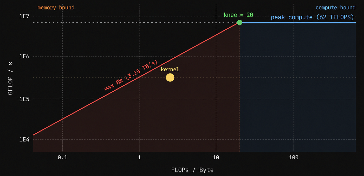
• The roofline model says every processor has two ceilings ,a peak compute throughput (FLOP/s) and a peak memory bandwidth (bytes/s). Their ratio is the machine’s ridge point/knee. If your workload’s arithmetic intensity is below that ridge point, you’re memory-bound: the compute units sit idle waiting for data to arrive. Adding faster cores won’t help. If it’s above, you’re compute-bound: the memory is fine, you just need faster cores for more FLOPS.

Roofline Model — Courtesy of BrrViz

For LLM decode (one token at a time), arithmetic intensity is tiny. To see why, take one of the FFN weight matrices: it’s 5632x2048 floats, about 11 million values. To multiply one token’s activations (a vector of 2048 floats) against that matrix, you do roughly 11 million multiply-accumulate operations. But you also had to load all 11 million weights from memory to do it. That’s roughly 1 FLOP per byte, far below the ridge point of any modern processor. The compute units finish their work and then sit idle, waiting for the next batch of weights to arrive from RAM.

Decode: 1 token × weight matrix
  memory loaded  : 11M floats  (~44MB)
  FLOPs done     : ~11M
  arithmetic intensity ≈ 1 FLOP/byte   ← deep in memory-bound territory

For prefill (processing the full input prompt at once), the picture changes. Now you’re multiplying a matrix of token activations — say 64 tokens ,against the same weight matrix. You still load the weights once, but now you do 64× more math with the same bytes.

Prefill: 64 tokens × weight matrix
  memory loaded  : 11M floats  (~44MB)   ← same as decode
  FLOPs done     : ~0.7B
  arithmetic intensity ≈ 64FLOPs/byte  ← much closer to compute ceiling

Same weights, same memory cost. But the compute is now spread across 64 rows instead of 1. That’s why TTFT and decode respond so differently to the same optimization — they’re hitting different parts of the roofline.

Quantization: The Model Doesn’t Run on INT4

There are many quantization formats out there: Q4_0, Q4_1, Q5_K, Q8_0, and more. They all make the same basic trade-off: fewer bits per weight means smaller file, less RAM, faster memory transfers, and some loss of precision. Tiny Llama 1.1B uses Q4_K for most weight matrices and Q6_K for a smaller set of more sensitive ones (the attention output and FFN down projections), where the extra precision is worth the cost.

Now here’s something that surprises people: the weights are stored in 4-bit format, but the model doesn’t actually compute in 4-bit.

To understand why, you need to know what quantization actually does to a number.

A 32-bit float can represent values across an enormous range with high precision. A 4-bit integer can only hold 16 distinct values: 0 through 15. So how do you squash a float into 4 bits without losing everything?

You divide the weights into small blocks say, 32 values at a time and for each block you find the minimum and maximum value. Those two numbers define the range the block needs to represent. Every weight in the block is then expressed as an integer from 0 to 15, mapping linearly across that range.

One block (32 weights on disk):
┌────────────────────────────────────────────────────┐
│  min: -0.5   max: 0.8   (stored once per block)    │
│  scale = (max - min) / 15                          │
├──────┬──────┬──────┬──────┬──────┬─────  ...  ─────┤
│  9   │  14  │  2   │  15  │  10  │       ...       │
│ 4bit │ 4bit │ 4bit │ 4bit │ 4bit │                 │
└──────┴──────┴──────┴──────┴──────┴─────────────────┘

Each 4-bit integer is meaningless on its own. It only becomes a usable float when you apply the block’s scale and min at compute time:

dequantized = q * scale + min

Concretely, say a block spans min = -0.5 to max = 0.8, and one of the weights is 0.3:

scale     = (0.8 - (-0.5)) / 15 = 0.0867
quantized = round((0.3 - (-0.5)) / 0.0867) = round(9.23) = 9

That single weight is now stored as the integer 9 , 4 bits instead of 32. The scale (0.0867) and min (-0.5) are stored once per block. To recover the original value at compute time:

dequantized = 9 * 0.0867 + (-0.5) = 0.28

Not exactly 0.3, but close. The error is the price you pay for the compression.

This also handles negative weights cleanly. A weight of -0.5 maps to 0, and 0.8 maps to 15. The full signed range of the block fits into 16 buckets.

Q4_K and Q6_K are more sophisticated variants of this, they use a two-level scaling scheme (a scale-of-scales) for better accuracy, but the core idea is identical.

At a high level, it’s the same principle as any compression algorithm:

FP32 weights  →  compress (quantize)  →  4-bit storage
4-bit storage →  decompress (dequantize)  →  FP32 for compute

The difference from general-purpose compression is that this is lossy . You don’t get the exact original value back. But for neural network weights, a small amount of precision loss turns out to matter very little in practice.

This is why quantization is a memory optimization, not a compute optimization. You fit a larger model in RAM and transfer fewer bytes from memory to the compute units. But the compute itself still happens in floating point.

Every production matmul GEMM dequantizes each block on the fly, right before accumulating the products. Now that you understand the roofline, you can see exactly why this matters: if we’re memory-bound, anything that reduces bytes in flight directly raises throughput.

Mental Model

So far we’ve covered the scaffolding: how the model is laid out on disk, how it gets mapped into memory, how the weights are quantized, and the two metrics, TTFT and decode — that every optimization will be judged against. Now we’ll put it all together and build a mental model of exactly what happens during inference — just the structure, no details yet.

There are roughly three steps:

// step 1: load weights into memory
transformer();
prompt = "Migrate entire codebase from typescript to assembly";

// step 2: prefill — process the entire prompt in one forward pass
tokens = tranfsormer.tokenize(prompt);
first_token = transformer.forward(tokens);
tokens.append(first_token);

// step 3: decode — generate one token at a time
while tokens.last != END_TOKEN:
    next_token = transformer.forward(tokens);
    tokens.append(next_token);

Every transformer.forward call is the same thing: run each of the 22 decoder blocks serially. Each block applies a series of mathematical operations:rms_norm, matmul, softmax, silu — using that layer’s weights, and passes its output to the next block. Where the costliest operation inside every block is matmul, by a large margin.

This means there are two knobs that control how fast inference runs:

• How fast weights load: fewer bytes to move means less time blocked on memory
• How fast matmul runs: it dominates the compute inside every block

Every optimization in this article tries to play around with these two knobs.

The Baseline

Now let’s see what happens when we keep everything as simple as possible.

Weights are loaded and dequantized eagerly at startup: every Q4_K/Q6_K matrix is unpacked into a plain FP32 array before the first token is ever generated. The 700MBmodel balloons to ~2.8GBin RAM. Simple — but the CPU now streams 4× more data through cache than necessary on every forward pass and model now occupies a lot of space in memory.

Matmul is just a simple naive triple loop:

for i in 0..M:
    for j in 0..N:
        acc = 0
        for k in 0..K:
            acc += A[k][i] * B[k][j]
        C[i][j] = acc

The inner loop over k accesses B[k][j] by stepping through memory in a pattern that jumps N elements forward each time — which is not how the data is laid out. With K=2048 and N=5632, you're skipping thousands of floats between each access. The CPU's prefetcher can't predict it. Cache lines get loaded, used for one value, and evicted before the next column access can reuse them.

Courtesy of Ryan Pégoud

Running this on TinyLlama 1.1B with a 512-token prompt:

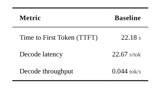
Profiling show that the CPU is running at 0.98 instructions per cycle. Almost exactly 1. A well-optimized loop should be 3 to 4 (CPU Pipelining). The processor is executing one instruction and then stalling, waiting for memory just cause the data isn’t in cache.

Optimization 1: Cache Tiling

To understand what tiling fixes, you need a concrete picture of what a cache miss actually costs.

Your CPU has three levels of cache sitting between it and main memory:

L1 cache :  32 KB  —  ~4 cycles to access
L2 cache : 256 KB  —  ~12 cycles to access
L3 cache :   3 MB  —  ~40 cycles to access
DRAM     :   8 GB  —  ~200 cycles to access

When the CPU needs a float that isn’t in L1, it checks L2, then L3, then finally goes to DRAM. That last step, a full cache miss to DRAM — costs 200 cycles. For one float. While the CPU is waiting, the pipeline stalls. This is exactly what was happening: 0.98 IPC, one instruction executed, then a ~200 cycle stall while the next chunk of the weight matrix arrives from RAM.

The naive matmul makes this inevitable. Ideally, we’d like to load each segment of data only once and perform all the operations in which they are used before dropping them from memory.

Tiling does exactly this(also called blocking). Instead of iterating over the full K dimension at once, you break A, B, and C into small square tiles that fit comfortably in L1 or L2 cache. You work on one tile at a time: load a tile of A, a tile of B, accumulate into a tile of C, then move to the next. The key insight is that within a tile, you reuse the same data across many multiply-accumulate operations — so the cost of fetching it from memory gets amortized.

Courtesy of Ryan Pégoud

The code changes the loop structure to walk through tiles first:

for ii in 0..M step TILE:
    for jj in 0..N step TILE:
        for kk in 0..K step TILE:          // tile over K
            for i in ii..ii+TILE:
                for j in jj..jj+TILE:
                    acc = C[i][j]
                    for k in kk..kk+TILE:  // inner loop now fits in cache
                        acc += A[k][i] * B[k][j]
                    C[i][j] = acc

Same six loops. Same arithmetic. But now the inner k loop only walks TILE_SIZE elements in B's column — a distance that fits in L1. The cache lines fetched for this tile get reused across all the i and j iterations within the tile, instead of being evicted before the next access.

I honestly didn’t expect this to make such a large difference. It’s a loop reorder — no new math, no new hardware, no vectorization. Just a different traversal order.

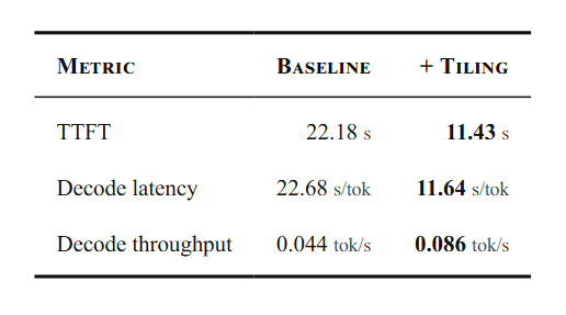
2× faster. Purely from keeping data in cache.

the algorithm’s memory access pattern matters more than the algorithm itself.

Optimization 2: SIMD — A Lesson in Expectations

After tiling cut runtime in half, the natural next step seemed obvious: vectorize the inner loop with SIMD.

SIMD (Single Instruction, Multiple Data) lets the CPU batch a chunk of data into wide registers and apply the same operation across all of it in a single step, instead of one number at a time. AVX2 is the instruction set (intrinsics) that exposes this on the i3–7100: its 256-bit registers hold 8 floats, so one instruction multiplies all 8 at once. In theory, the inner loop could run 8× faster.

// each output row of C
for (int i = 0; i < M; i++) {
    // contiguous reads, no big jumps                             
    pack_panel(A, i, packedA); 
    // 8 columns at a time                           
    for (int j = 0; j < N; j += 8) {    
        // 8 accumulators set to 0                  
        __m256 acc_vec = _mm256_setzero_ps();             
        for (int k = 0; k < K; k++) {
            // copy A[k] into all 8 lanes
            __m256 a_vec = _mm256_broadcast_ss(&packedA[k]); 
            // load B[k][j .. j+8] 
            __m256 b_vec = _mm256_loadu_ps(&B[k][j]);   
            // multiply + add, 8 lanes, 1 instruction      
            acc_vec = _mm256_fmadd_ps(a_vec, b_vec, acc_vec); 
        }
        // write 8 results back
        _mm256_storeu_ps(&C[i][j], acc_vec);               
    }
}

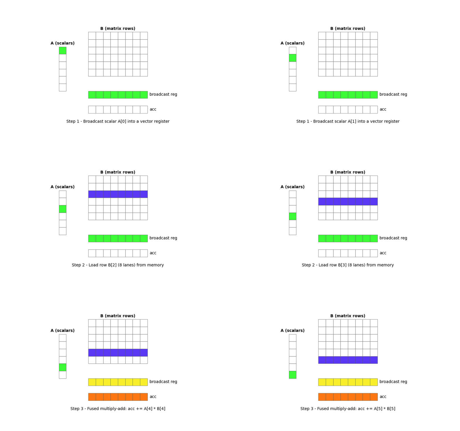
SIMD — Step By Step Visualization

Clean implementation. AVX2 FMA instructions firing. Should be fast.

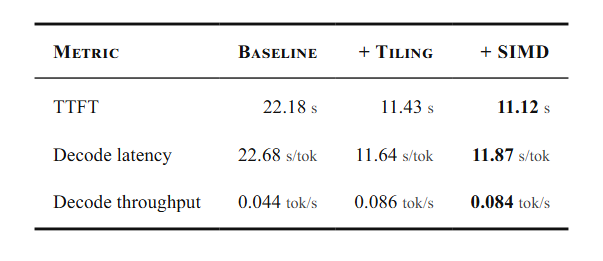
3%. Essentially nothing.

The roofline model predicted this exactly. The i3–7100’s memory bandwidth is ~37 GB/s. Its peak AVX2 throughput is ~230 GFLOP/s. The ridge point, bandwidth divided by peak compute — is around 6 FLOP/byte. Our matmul is running at roughly 1 FLOP/byte. We are nowhere near the compute ceiling.

This means that the ALUs are already sitting idle doing nothing, just waiting for memory to load. Making them process 8 floats simultaneously when they were already idle changes nothing — the bottleneck is still how fast data arrives from RAM.

This is a brutal but important result I had to internalize after spending an entire day writing beautiful vectorized code, profiling it, watching it execute — and it makes no measurable difference. Because the true bottleneck is not what I optimized.

Measure first. Optimize second.

Optimization 3: KV Cache

Let’s optimize our true bottleneck. Here’s a good analogy for what was happening without a KV cache.

Imagine you’re reading a book, and every time you encounter a new word, you go back and re-read the entire book from page one before continuing. That’s what the baseline decoder was doing. For each new token it generated, it re-projected every previous token through the K and V weight matrices, effectively re-reading the entire context from scratch — even though those projections hadn’t changed at all.

The KV cache eliminates this. At startup, you pre-allocate a single contiguous arena in memory sized for the maximum sequence length:

KV arena layout:
┌──────────────────────────────────────────────────────────────┐
│  Layer 0  K  [ head_dim × kv_heads × max_seq_len ]          │
│  Layer 0  V  [ head_dim × kv_heads × max_seq_len ]          │
├──────────────────────────────────────────────────────────────┤
│  Layer 1  K  ...                                             │
│  Layer 1  V  ...                                             │
├──────────────────────────────────────────────────────────────┤
│  ...  (22 layers total)                                      │
└──────────────────────────────────────────────────────────────┘

During prefill, K and V for every token and every layer are computed and written into their slots. On each subsequent decode step, you only compute K and V for the single new token, append it into the next slot, and attend over the full cached sequence. The projection work for everything that came before is free.

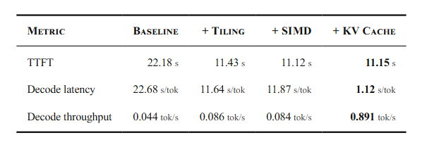
Decode improves by 10.6×. TTFT barely changes and that’s expected. The KV cache only helps decode. During prefill, the cache is cold: there’s nothing stored yet, so every token’s K and V still has to be computed from scratch. It’s not that the cache failed during prefill, it’s that it simply hasn’t accumulated anything yet. The first token is always the most expensive.

This is the single biggest behavioral change in the whole series. Tiling and SIMD were trying to speed up each matmul — they were fighting a memory-bandwidth wall, making already-idle ALUs work slightly harder. This optimization basically reduces the amount of redundant work the ALUs were doing by simply caching the results.

Real production systems like vLLM go further with paged attention — managing the KV cache in fixed-size pages instead of a single contiguous arena, similar to how an OS handles virtual memory. This avoids fragmentation when serving many users with different context lengths simultaneously. But that’s a story for another time.

Optimization 4: Quantized Kernels

Remember what the baseline did at startup: it walked every weight tensor in the GGUF file and eagerly dequantized all of it, every Q4_K and Q6_K block — into full FP32 float arrays, allocating fresh memory to hold the result. By the time main() returned from the constructor, the 700MB model file had been unpacked into roughly ~2.8GB of floats sitting in RAM. Every matmul then operated on those floats directly.

This made the matmul simple.But it also meant longer startup times and larger memory bandwidth between memory and the CPU.

The fix is to stop dequantizing upfront and instead fuse dequantization directly into the matmul, basically make it lazy. The weights stay in their compact Q4_K/Q6_K format in memory, exactly as they appear in the file. The matmul kernel reads one block at a time, unpacks just those 32 values into a small scratch buffer, and immediately uses them for the dot product accumulation:

// Quantized matmul (one output row m, over all K blocks):
for each block b in 0..K/32:
    scratch[0..31] = dequantize(W_row_m[b])   // unpack 32 × 4-bit → 32 floats
    for each column n:
        C[m][n] += dot(scratch, X[b*32..(b+1)*32][n])

The scratch buffer is 32 floats, 128 Bytes, fits entirely in L1 cache. You unpack a block, consume it immediately across all output columns, and move on. The 4-bit weights are loaded once and never written to a large intermediate float array. No upfront allocation. No ~2.8GB in memory.

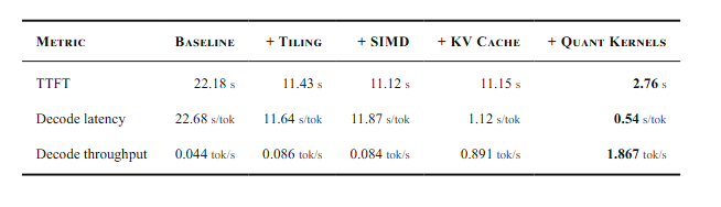
A 4× improvement on TTFT, the biggest single jump in the whole series.

The reason is straightforward now. The FFN up/down projection matrices are 5632x2048 weights each. In FP32, one matrix is ~44MB. In Q4_K, the same matrix is ~11MB. Every time the matmul sweeps through those weights, it now moves 4xfewer bytes across the memory bus. We’re still memory-bound, but we’ve moved up towards the roofline ceiling, the same bandwidth now delivers 4x more weights per second.

This is the point where quantization stops being just a storage trick and starts being a genuine runtime optimization. Same arithmetic, fewer bytes in flight.

Optimization 5: CUDA — Moving to the GPU

Everything so far has been CPU-only. Now we move compute to the GPU.

A quick GPU mental model

A GPU runs thousands of tiny threads at once, organized into thread blocks where each block is a group of threads (here, 256) that run together. Each block is arranged in a grid like fashion all executing in parallel.

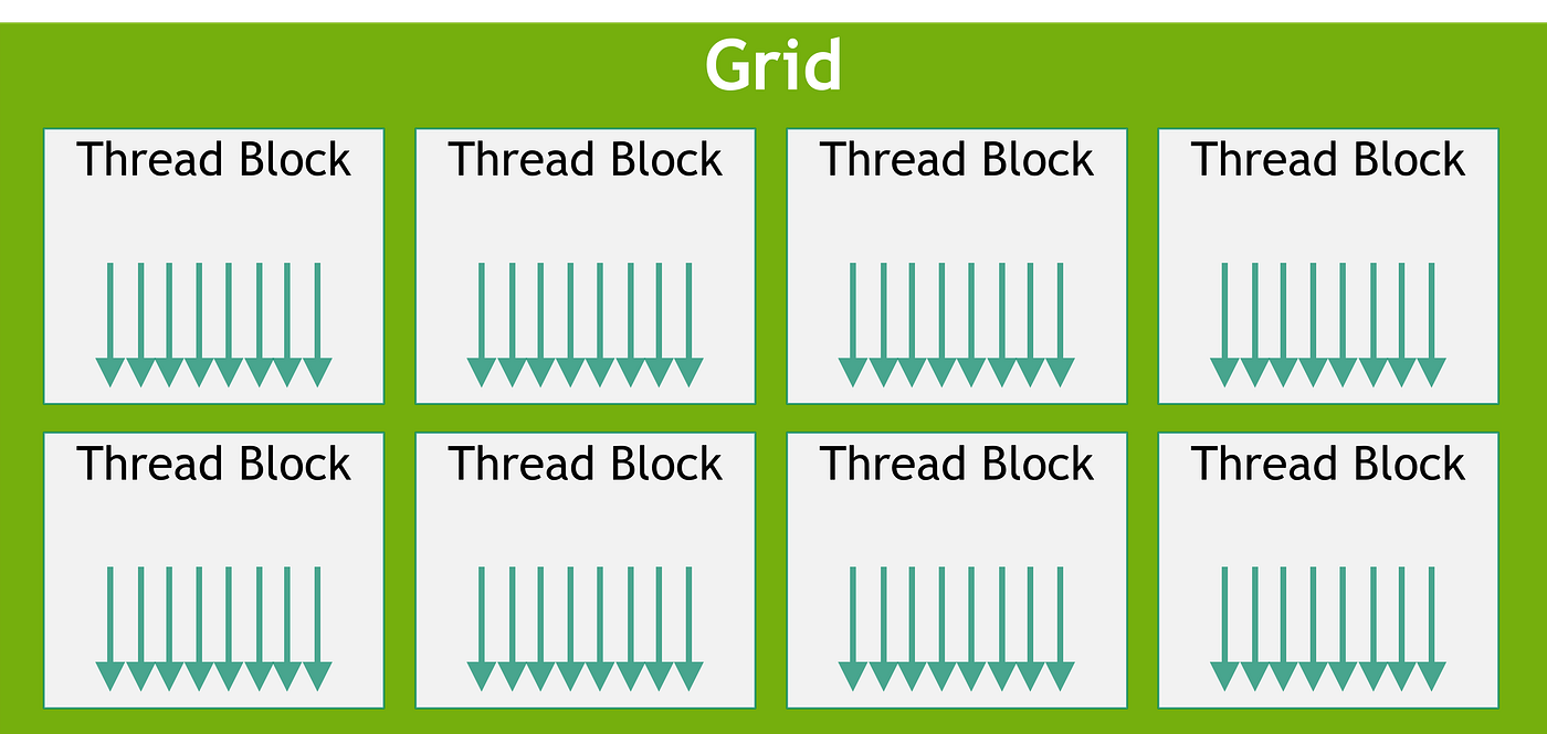
Courtesy of Nvidia

Each thread block can share a small patch of fast on-chip shared memory (analogous to the CPU L1 cache). Everything else lives in global memory: GPU’s VRAM (analogous to CPU RAM), large by comparatively slow. The game is the same one we’ve been playing on the CPU all along, keep hot data in fast memory and minimize trips to slow memory.

The CPU and GPU are separate chips with separate memory. They communicate over a PCIe bus and that link is the first thing that can go badly wrong.

The memory movement problem

The 750 Ti sits on a PCIe 3.0 x16 slot. The theoretical bandwidth of that bus is ~16 GB/sin each direction. The GPU’s own GDDR5 memory runs at ~86 GB/s internally. The moment you need to move data between CPU and GPU, you’re bottlenecked by PCIe. A 5× slowdown compared to what the GPU can do on its own memory.

A naive GPU port, upload activations to the GPU, run cublasSgemm (A CUDA Matmul), download the result, repeat per layer, would be catastrophically slow. The decode path runs ~100matmuls per token across 22 layers. Each one would require two PCIe transfers: one to upload the input, one to download the output. At even a few MB per transfer, PCIe would dominate the runtime completely.

Naive (wrong) approach:
for each layer:
    cudaMemcpy(x_gpu ← x_cpu)          // PCIe upload
    cublasSgemm(w_gpu, x_gpu → y_gpu)   // GPU compute
    cudaMemcpy(y_cpu ← y_gpu)          // PCIe download
    ... repeat 100+ times per token

The fix is to never come back. Everything stays on the GPU:

Correct approach:
startup:  
  Step 1: upload all weights to GPU VRAM once
  Step 2: allocate KV cache in GPU VRAM
  Step 3: allocate activation buffers in GPU VRAM
per token: 
  Step 1: run entire forward pass on GPU
  Step 2: cudaMemcpy just the final logits back to CPU (32,000 floats, ~128KB)

Weights are uploaded once, a one-time cost at startup, not on every token. The KV cache lives in VRAM. Activations are computed and consumed entirely on-device. The only PCIe transfer per token is 128KB of logits at the very end.

Why a plain matmul kernel isn’t enough

Even with data resident on the GPU, you can’t just use cublasSgemm for the quantized weights. cuBLAS operates on FP32 or FP16 matrices. Your weights are in Q4_K format, 4 bits per value with block-level scales. You need a custom kernel that understands the quantization format, something similar to the CPU quantized kernel we built.

The Cuda Quantized Kernel

So we write our own. A group of 256 GPU threads takes one compressed weight block, and each thread unpacks a single value into fast on-chip shared memory. As soon as the block is unpacked, the same threads read from the shared memory and use those values directly in the dot product — the unpacked weights never get written back out to slow global memory:

Each thread block handles one output tile:
  load weight block (packed bytes) from global memory
  256 threads cooperate: each thread dequantizes its element into shared mem
  accumulate: each thread computes its contribution to the dot product
  write result to output in global memory

No intermediate FP32 weight matrix is ever materialized. The dequantization and multiplication happen inside the same register file, on the same data, without additional memory traffic.

The Fused Attention Kernel

The attention forward pass has a similar problem. The standard approach writes a full [seq_len × seq_len] score matrix to global memory, then reads it back for the softmax, then reads it again for the weighted sum of V. Three passes over a matrix that can be large.

The fused kernel eliminates the score matrix entirely using online softmax , an algorithm that computes the numerically stable softmax and weighted V accumulation in a single pass, maintaining a running max and sum:

// Grid : (q_heads, seq_len)  — one block per (head, query position)
// Block: head_dim threads    — one thread per element in the head
Each block:
  load Q[h, q_pos] → shared memory
  single pass over key positions 0..q_pos:
      score = scale × dot(Q, K[k])   // QK^T
      update running max, softmax denominator
      accumulate weighted V[k]
  write output → global memory
  (score matrix never touches global memory at all)

What nvprof actually shows

Running nvprof (Nvidia Benchmarking Tool) on the full inference gives a precise breakdown of where GPU time goes:

GPU activities:
  80.4%  4.89s   matmul_q4k_kernel    1206 calls  avg 4.1ms
  17.2%  1.05s   matmul_q6k_kernel     189 calls  avg 5.5ms
   2.0%  124ms   CUDA memcpy HtoD      232 copies  avg 534µs
   0.15%  9.3ms  fused_attn_kernel     198 calls  avg 47µs
   0.03%  1.9ms  rms_norm_kernel       405 calls  avg 4.6µs
   0.02%  933µs  add_kernel            396 calls
   0.01%  754µs  silu_kernel           198 calls
   0.01%  627µs  CUDA memcpy DtoH       40 copies
API calls:
  95.9%  5.93s   cudaFree             2404 calls  avg 2.5ms  ← !!
   2.4%  151ms   cudaMemcpy           1856 calls
   1.0%   64ms   cudaMalloc           2605 calls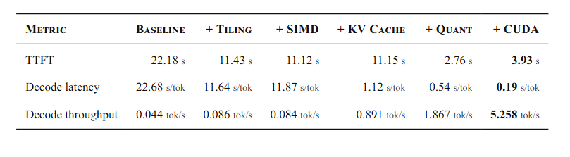

Decode is a clear win, 2.8x faster — but TTFT moved the wrong way: 3.93s versus 2.76s on CPU. The nvprof breakdown above explains where the time actually goes.

The quantized matmul kernels dominate GPU activity, 97.6% of GPU time combined — which is exactly right. That’s the real work.

The fused attention is remarkable: 198 calls across all decode steps averaging 47µs each. Total attention time: 9.3ms. On the CPU it was a meaningful fraction of runtime; here it’s noise.

So why is TTFT slower on GPU when it’s faster at everything else? It’s not a GPU limitation, it’s two avoidable costs in my own implementation stacking up.

Cost 1: the embedding lookup still runs on the CPU. This happens right at the start of every forward pass. It’s the very first step, before any of the 22 decoder layers run, turning the raw token IDs into the input vectors the layers operate on. The embedding lookup itself is simple: each token is just an integer ID, and the model stores a big table with one learned vector per vocabulary entry. The lookup grabs that token’s row and uses it as the token’s starting vector. In this model the rows are stored quantized, and that dequantization was never ported to a GPU kernel, so for every prompt token the data bounces across the PCIe bus:

// weights live on GPU including the embedding table...
transformer.device(cuda)               
tokens = transformer.tokenize(prompt)

// ...but embed() was never ported, so every token round-trips across PCIe:
for each token in tokens:
    // PCIe: GPU → CPU
    cudaMemcpy(row_cpu ← emb_table_gpu[token])  
    // CPU unpacks
    row_vec = dequantize(row_cpu)               
    // PCIe: CPU → GPU
    cudaMemcpy(input_vecs_gpu ← row_vec)        
    // 2 PCIe transfers per token
    input_vecs.append(row)  

first_token = transformer.forward_(input_vecs)   // GPU finally starts

Cost 2: memory is allocated and freed on every layer. Each decoder layer calls cudaMalloc/cudaFree for its scratch buffers, and this is a big systems no no — never allocate and free on a hot path, cause allocating and deallocating is costly memory operation.

Both costs are easy to fix, move the embedding lookup onto the GPU, and allocate a scratch memory arena like we did for the KV Cache, once instead of freeing it every layer. But left as-is, it’s a textbook example of where hidden PCIe round-trips and allocator stalls quietly eat your time.

What This Whole Journey Actually Looks Like

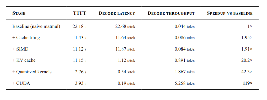
From 22.67s per token to 190ms. Same model, same machine. Every bit of that speedup came from how the code touches memory.

Where This Goes Next

Everything here is running on a single device with a single sequence. The real frontier is different:

**Paged Attention (vLLM)**: a virtual-memory-like approach to the KV cache paged, reclaimed, and shared across requests.

**Triton Matmul Kernels**: our hand-written CUDA matmul kernels dominated the profile, 97.6% of GPU time. This blog builds the same matmul as a Triton kernel instead of raw CUDA, less boilerplate, and it autotunes for you.

**Multi-GPU inference and distributed training**: Explains how large scale frontier models are trained, covers data and model parallelism across devices.

And if you want to see the memory movement of a GPU, **BrrrViz** is an interactive visualizer for how data moves through the GPU Memory Hierarchy, gives a better understanding of the compute and memory arguments discussed here.

The crossover of ML and systems is far more interesting than it gets credit for. Most of the attention goes to the models, the architectures, the benchmarks, but the layer underneath all of that, the part that decides whether a model runs in two seconds or two minutes, is its own quiet, fascinating world. The math got solved years ago. The systems are what actually puts the model in your hands.

This project is available on **GitHub**. Each optimization lives on its own branch, building directly on top of the one before it: NAIVE → TILING → SIMD → KV_SIMD → KV_QUANTIZED → KV_CUDA.

So you can check out any stage in isolation and see exactly what changed from the previous step. Each branch also carries its own benchmarks, profiling data, and detailed stats, so you can dig into the numbers behind every speedup yourself rather than taking mine at face value.