SE(3)-Transformer for molecular property prediction

Authors: Anuya Welling, James E. T. Smith, Diptorup Deb, Mukhil Azhagan Mallaiyan Sathiaseelan, Yao Liu, Phani Vaddadi, Jatinkmar parmar and Vish Vadlamani Knowledge level: Intermediate

The SE(3)-Transformer is a graph neural network that uses a variant of self-attention for 3D points and graphs processing. This model is equivariant under continuous 3D roto-translations, which means that when the inputs (graphs or sets of points) rotate in 3D space (or more generally experience a proper rigid transformation), the model outputs either stay invariant or transform with the input.

In the SE(3)-Transformer model, both training and inference are framed as regression tasks over a set of molecular properties. These include parameters such as μ, α, HOMO, LUMO, gap, R², ZPVE, U₀, U, H, G, and Cv, along with their atom-wise counterparts and rotational constants (A, B, C).

While the full physical interpretation of many of these quantities is best left to subject matter experts, this tutorial focuses on a few key electronic properties that are commonly used in molecular modeling. HOMO (Highest Occupied Molecular Orbital) refers to the highest energy level that is still occupied by electrons. LUMO (Lowest Unoccupied Molecular Orbital) is the lowest energy level that does not contain electrons and is available for occupation. The HOMO-LUMO gap, often simply called “the gap”, is the energy difference between these two orbitals and is an important indicator of a molecule’s electronic and chemical behavior.

In drug discovery, SE(3)-Transformer models predict molecular properties that matter for real biological behavior. A good drug must bind strongly to its target, avoid off-target reactions, and remain stable in the body while being reactive at the right site.

HOMO and LUMO capture this balance. They indicate a molecule’s tendency to donate or accept electrons, which influences how it reacts with protein amino acids and whether it could be toxic. The HOMO-LUMO gap acts as a proxy for reactivity — too small can mean instability and side effects, while too large can mean inactivity. Poor reactivity often leads to drug failure, even when binding looks promising.

For more information

To find out more about DGL, SE(3)-Transformers, and AMD ROCm performance benchmarks, see the following blogs:

Prerequisites

This tutorial was developed and tested using the following setup.

Hardware requirements

Note: This tutorial has been tested and validated on AMD Instinct MI300X GPUs. For the official list of supported GPUs, see the DGL Compatibility Documentation. For performance metrics on AMD Instinct GPUs, see the SE(3)-Transformer performance report blog.

Software requirements

AMD validates and publishes DGL images with ROCm backends on Docker Hub. The following table shows the validated software stack configurations:

Set up the SE(3)-Transformer environment

In this tutorial, you will work on the prebuilt ROCm DGL image as an example. You can also use other validated DGL images from the table above.

Step 1: Launch the Docker image

Launch the Docker container. Replace /path/to/workspace with the full path to the directory on your host machine where you want to clone the DeepLearningExamples code and run the notebook. Choose the image tag from the validated Docker images table above that matches your desired configuration.

dockerrun-it--rm--privileged\ --network=host\ --device=/dev/kfd\ --device=/dev/dri\ --group-add=video\ --ipc=host\ --cap-add=SYS_PTRACE\ --security-optseccomp =unconfined\ -v/path/to/workspace:/workspace\ -w/workspace\ <IMAGE_TAG>

Note: This command mounts your host directory to /workspace in the container. Ensure the notebook file is in this directory or upload it after Jupyter starts. The remaining steps should be run inside the Docker container. Save the URL (and token, if shown) from the terminal output to access JupyterLab from your browser.

For example, to use ROCm 7.0.0 with PyTorch 2.7.1:

dockerrun-it--rm--privileged\ --network=host\ --device=/dev/kfd\ --device=/dev/dri\ --group-add=video\ --ipc=host\ --cap-add=SYS_PTRACE\ --security-optseccomp =unconfined\ -v/path/to/workspace:/workspace\ -w/workspace\ rocm/dgl:dgl-2.4.0.amd0_rocm7.0.0_ubuntu22.04_py3.10_pytorch_2.7.1

Step 2: Install and launch Jupyter

Inside the Docker container, install Jupyter and the visualization packages used by this notebook:

Start the Jupyter server:

jupyter-lab--ip= 0.0.0.0--port= 8888--no-browser--allow-root

Note: Ensure port 8888 is not already in use on your system before running the above command. If it is, you can specify a different port by replacing --port=8888 with another port number, for example, --port=8890.

Step 3: Open the notebook

Once JupyterLab is running, open your browser and go to the URL shown in the terminal (typically http://localhost:8888). In the file browser, navigate to DGLPyTorch/DrugDiscovery/SE3Transformer/ and click se3transformer.ipynb (or this intro notebook) to begin. Alternatively, you can upload this notebook to your Jupyter lab via the upload button in Jupyter.

Two ways to use this notebook

This notebook supports two modes:

To select a mode, set USE_PRETRAINED = True (for inference) or USE_PRETRAINED = False (for training) in the configuration cell below.

Note: Run the rest of this notebook in Jupyter by executing the cells.

Loading the dependencies and repository

This section explains how to download and install the required code and dependencies.

Install dependencies

!pipinstallplotlytorchinfordkitpy3Dmol

What happens next?

First, choose between inference or training mode.

Depending on which setting you choose, the next steps vary somewhat:

Imports for training and evaluation

These imported modules set up the full SE(3)-Transformer training and evaluation pipeline on the QM9 molecular dataset. They cover data loading, distributed training, optimization, logging, and inference.

Download the pretrained model from Hugging Face

If you are using pretrained mode ( USE_PRETRAINED = True), the model_qm9_100_epochs.pth checkpoint must be available locally. This checkpoint is hosted on the Hugging Face Hub. To download it, follow these steps:

1. Install the Hugging Face Hub client using pip install huggingface_hub.
2. Log in to Hugging Face (recommended for gated or rate-limited access). Run huggingface-cli login in a terminal and enter your token from huggingface.co/settings/tokens.
3. Download the model into the current directory with:

• huggingface-clidownloadamd/se3_transformersmodel_qm9_100_epochs.pth — local-dir.

The cell below automatically runs these steps when USE_PRETRAINED is True.

Dataset and model setup

Start by loading the QM9 molecular dataset using QM9DataModule, which handles data preprocessing, batching, and splitting for training and evaluation. Next, initialize the SE(3)-Transformer model (SE3TransformerPooled) with input, edge, and output fibers that define how geometric and feature information flows through the network. Finally, define the L1 loss ( nn.L1Loss) - a simple yet effective choice for molecular property regression tasks.

Inspecting the molecules

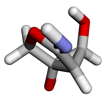
Before diving into training, it’s helpful to visually inspect the molecules from the QM9 dataset.

Review one of the molecules in the dataset:

Basic graph information

--- BASIC INFO --- Nodes: 14 Edges: 28

The molecule is represented as a graph with 14 nodes corresponding to atoms and 28 edges representing atom-atom interactions. Edges are constructed based on interatomic proximity rather than explicit chemical bonds.

Node features (ndata)

Each node (atom) is associated with geometric and chemical features.

Atomic positions

Key: pos Shape: (14, 3) Dtype: torch.float32 tensor([[ 0.6781, -0.0583, 0.7324], [-0.1432, 0.3297, -0.3889], [-1.5010, -0.2886, -0.2937], ...])

Each row represents the 3D Cartesian coordinates [x,y,z] of an atom in the molecule.

Atomic attributes

Key: attr Shape: (14, 11) Dtype: torch.float32 tensor([[0., 0., 0., 1., 0., 8., 0., 0., 0., 0., 1.], [0., 1., 0., 0., 0., 6., 0., 0., 0., 0., 2.], [0., 1., 0., 0., 0., 6., 0., 0., 0., 0., 0.], ...])

Each row encodes atom-specific properties, such as atomic type and related categorical or numerical descriptors, which allow the model to distinguish between different elements.

Edge features (edata)

Edges capture pairwise relationships between atoms.

Edge Attributes Key: edge_attr Shape: (28, 4) Dtype: torch.float32 tensor([[1., 0., 0., 0.], [1., 0., 0., 0.], [1., 0., 0., 0.], ...])

Each row represents a feature vector associated with an edge, typically encoding distance-based or radial information used to model interatomic interactions.

RAW values of HOMO, LUMO, and GAP

The raw values of HOMO, LUMO and GAP in eV is as follows.

HOMO (Highest Occupied Molecular Orbital) energy LUMO (Lowest Unoccupied Molecular Orbital) energy GAP (gap between HOMO and LUMO)

View the model summary

Quickly inspect the SE(3)-Transformer architecture using torchinfo.summary, which prints a detailed overview of each layer, its input/output shapes, and the number of parameters. This helps you verify that the model has been built correctly before training.

Part A: Training pipeline (optional)

Use this code to configure the training pipeline.

Note: If USE_PRETRAINED is set to True, the training cells below will be skipped, and you'll proceed directly to inference.

Logging and callbacks

Train

With everything configured, you’re ready to kick off training. The train() function orchestrates the entire training loop - running forward and backward passes, computing losses, updating parameters, and periodically evaluating the validation set. It uses the dataloaders, callbacks, and logger you set up earlier to track progress, log metrics, and manage learning rate schedules throughout the training process.

Visualizing the training progress

After training, you can visualize and analyze the logged results. Import Plotly for interactive plotting and dllogger to access the saved training logs. Flushing the logger ensures all metrics have been written to disk before loading them.

This step parses and organizes the logged training data from dllogger_results.json. It reads the file line by line, cleans up any malformed entries, and filters out records without valid steps. Each log entry is then grouped by its training step, extracting key metrics such as training loss, learning rate, and validation mean absolute error (MAE). The results are compiled into a tidy Pandas DataFrame, making it easier to visualize and analyze how model performance and learning dynamics evolved throughout training.

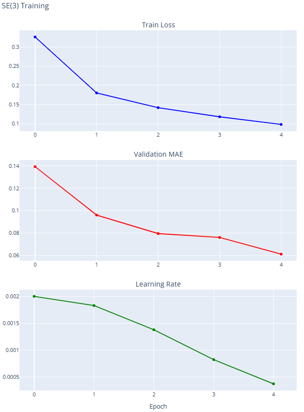
To get a clear picture of how training evolved, plot the key metrics over epochs using Plotly. The figure below displays training loss, validation MAE, and learning rate in separate subplots, making it easy to observe the model’s convergence and learning dynamics. Ideally, you should see the training loss and validation MAE steadily decreasing as the learning rate adjusts, giving quick visual confirmation that training progressed smoothly.

Here’s an example of what the output graph might look like:

Part B: Inference and evaluation

This section loads a trained model checkpoint and evaluates it on the test set.

Load the pretrained checkpoint

The following code loads the checkpoint you previously downloaded.

After this step, the model is ready for inference.

Post-inference analysis

Referring to the previous example, you can now inspect the molecule, examine its regression targets, and compare it with the prediction.

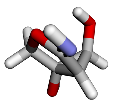
To obtain these values, run separate training and inference sessions for each task, specifying the --task argument as homo, lumo, or gap.

HOMO (Highest Occupied Molecular Orbital) energy

TARGET : tensor ([ 1.2334 ]) PREDICTION : tensor ([ 1.2236 ], dtype = torch . float16 )

LUMO (Lowest Unoccupied Molecular Orbital) energy

TARGET : tensor ([ 0.5246 ]) PREDICTION : tensor ([ 0.5127 ], dtype = torch . float16 )

Gap (Energy difference between HOMO and LUMO)

TARGET : tensor ([ - 0.0547 ]) PRED : tensor ([ - 0.1097 ], dtype = torch . float16 )

Conclusion

This notebook walked you through the end-to-end workflow for training and evaluating an SE(3)-Transformer model on the QM9 molecular dataset. You explored how to set up training configurations originally designed for CLI use, adapted them for an interactive Jupyter workflow, and visualized molecules directly from graph data to validate preprocessing. You then built and trained the SE(3)-Transformer, logged its performance, and used interactive plots to analyze key metrics like loss, MAE, and learning rate over time.

With the workflow now validated, this setup provides a strong foundation for scaling up experiments, benchmarking performance, and adapting the SE(3)-Transformer to more complex or domain-specific datasets.

Originally published at https://rocm.docs.amd.com.