From rank 46 to rank 3: training an embedding model for Data Lake table search

At Raiffeisen Bank Ukraine, we are building an internal LLM agent over the bank’s Data Lake. The promise is straightforward: a user asks a business question in natural language, English or Ukrainian, and the agent finds the right data, writes SQL, validates the query, and returns an answer.

The part that looks simple on the architecture diagram is the part that decides whether the product can be trusted. Before the LLM writes SQL, it must find the tables that can answer the question. If it finds the wrong tables, the rest of the pipeline can still look healthy. The SQL can be syntactically valid. Athena can run it. The final response can be formatted clearly. The answer can still be wrong.

That is worse than an error. A failed query tells the user something broke. A confident answer computed from the wrong table gives no obvious warning, and the user asked the agent precisely because they did not already know where the answer lived.

So table discovery became a correctness boundary for our text-to-SQL system. Then that boundary failed in a way we did not expect. Several card-transaction tables that should have been near the top of search results fell into positions 30, 40, and 50+. These were not obscure tables. They lived in different databases and represented different parts of the transaction data model. For questions like “show me card transactions,” they were exactly the kind of fact tables the agent had to find first.

One representative transaction table fell to rank 46.

That result changed the project. Until then, the work looked like a familiar enterprise RAG story: use a strong multilingual embedding model, improve table descriptions, generate synthetic questions, add hard negatives, fine-tune, and watch the metrics improve. Instead, the training signal that was supposed to make the model more precise had buried some of our most important tables.

The final model fixed the failure. On the held-out test set we used for the OpenAI comparison, the generic embedding model found the correct table in the top 10 only about half the time. Our fine-tuned BGE-M3 model found it almost nine times out of ten.

+-----------+-------------------------------+-------------------+
| Metric    | OpenAI text-embedding-3-large | Fine-tuned BGE-M3 |
+-----------+-------------------------------+-------------------+
| MAP@10    | 0.2853                        | 0.5919            |
| Recall@5  | 0.4197                        | 0.7983            |
| Recall@10 | 0.5146                        | 0.8838            |
| NDCG@10   | 0.3400                        | 0.6627            |
+-----------+-------------------------------+-------------------+

Those numbers made the text-to-SQL pipeline viable. But the interesting part is not that fine-tuning helped. The interesting part is why the obvious fine-tuning path failed, why iterative hard-negative mining made it worse, and why the fix was to stop trusting the closest neighbours.

In this article

1. Why a wrong table is worse than a failed query A text-to-SQL agent can produce a confident answer from the wrong data, and that makes table discovery a correctness boundary.
2. Why the catalogue cannot just be placed in the prompt A realistic table representation is large. Across thousands of tables, the catalogue is many millions of tokens.
3. Why table discovery is different from document retrieval The user is not looking for a paragraph with similar wording. They are looking for the place in the data model where an answer can be computed.
4. How we generated the training signal We used metadata, Claude-generated bilingual descriptions, synthetic questions, and LLM-classified hard negatives.
5. Why the obvious improvement made things worse Iterative hard-negative mining improved the aggregate number while burying critical transaction tables.
6. How hard negatives buried the right tables Dense clusters of similar transaction tables started pushing each other apart during contrastive training.
7. What fixed the model We changed negative mining to skip the nearest cluster siblings and train on the next band of confusing but safer candidates.
8. Why the final model was not one trick Priority weighting, duplicate handling, dynamic negatives, and per-priority evaluation made the fix stable.
9. How the model runs in production The embedding service runs on ECS Fargate, and the MCP server reranks the top results with Claude Sonnet using conversational context.
10. What I would take from this If your RAG target is a data asset rather than text, evaluate and train directly for that retrieval decision.

1. A wrong table is worse than a failed query

The opening failure is worth naming because it defines the stakes. A text-to-SQL agent does not fail only when SQL generation fails. It also fails when retrieval gives SQL generation the wrong starting point. In that case, the system can produce a valid query, run it successfully, and return a plausible answer that came from the wrong part of the Data Lake.

For a user, that is a dangerous failure mode. They usually cannot inspect the table selection, joins, and lineage before trusting the number. They asked the agent because they wanted help navigating the data model. If table discovery is wrong, every downstream step is built on the wrong foundation.

That is why the rank-46 transaction-table result mattered so much. It was not a cosmetic search-quality issue. It meant the agent could miss the obvious fact tables for a common business intent and still proceed as if nothing unusual had happened.

2. The catalogue is not the context

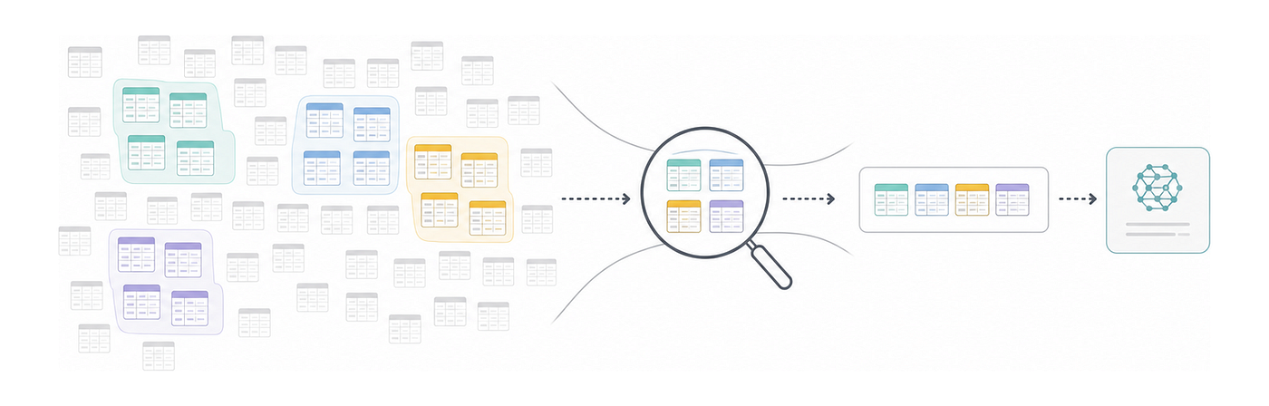
The full Data Lake is far too large for an LLM to inspect directly. It contains roughly 500 TB of data across about 40K tables. The agent does not search every table in the lake, but even the searchable business catalogue is around 7K tables across roughly 100 databases.

A useful table representation is not just a table name. To let an LLM reason about a table, we need a description, columns, types, categories, lineage hints, and enough context to distinguish it from similar tables. One table can easily approach a couple of thousand tokens. Across the searchable catalogue, that is on the order of 12–15 million tokens.

There is no practical context window where that belongs. Even if a future model accepted a prompt that large, sending the whole catalogue for every question would be slow, expensive, and bad for reasoning. The relevant schemas would be buried among thousands of irrelevant ones, and the LLM would still need to decide which tables matter.

This is the same reason long-context models do not remove the need for retrieval. Designing Large Language Model Applications [1] makes a useful distinction here: real production corpora are not needle-in-a-haystack tests with unrelated distractors. They contain related distractors, and related distractors are exactly what enterprise catalogues are full of. Agentic Design Patterns [2] frames the same point as context engineering: the input to an LLM should be a curated payload, not everything the system knows.

So the agent needs retrieval before reasoning. It needs a short, ranked list of candidate tables. Only then can the SQL-generation step start.

That retrieval layer is harder than it sounds because enterprise metadata is not a clean corpus of documentation. Table names carry local conventions: source-system prefixes, archive suffixes, historical variants, raw-layer names, integration-layer names, curated-layer names. Descriptions exist in Alation Data Catalog, but their completeness varies a lot from owner to owner. Some are detailed and maintained. Some are short. Some assume the reader already knows the local data model. Column names are abbreviated. Documentation switches between English and Ukrainian.

The data-platform literature says the same thing from the opposite direction. Architecting Data and Machine Learning Platforms [7] treats the catalogue as a first-class discoverability layer once a platform grows beyond a small number of datasets, while Data Quality Fundamentals [8] argues that lake-scale environments need automated, discovery-oriented metadata because static catalogue maintenance lags behind reality.

The obvious solution is semantic search. Embed every table description. Embed the user’s question. Return the nearest tables.

That is close enough to be useful and wrong enough to fail.

3. We were not searching for similar text

An embedding model turns text into a vector: a fixed-length list of numbers that makes similarity computable. If “card transactions last month” and “monthly card purchase volume” point in roughly the same direction, vector search treats them as similar. This is the basic mechanism behind many RAG systems.

For document retrieval, that abstraction often works well. A user asks about a vacation policy, and the system retrieves the vacation policy document. A user asks about a database setting, and the system retrieves a documentation page. The query and the target are both pieces of text, so the job is mostly text-to-text similarity.

Our target was different. We were not trying to retrieve text that sounded like the user’s question. We were trying to retrieve the table, or a small group of lineage-linked tables, where the answer could be computed.

That distinction changes the problem. A question like “card transactions for retail customers last month” is an intent. A table description is a description of a data asset. The right match is not “do these two strings mean the same thing?” It is “Does this table contain the data needed to answer this question, possibly after a join?”

That makes catalog metadata load-bearing for natural-language analytics. Modern Data Architecture on AWS [3] describes the common NL-to-SQL pattern as an LLM grounded by database, schema, and table definitions before it writes a query. If the grounding step picks the wrong table, the SQL can still be valid while the answer is wrong.

This makes relevance asymmetric. The question points at the table, but the table does not naturally point back at the exact question. It also makes the relevance composite. A real business question may need a transaction fact table, a customer dimension, and a product reference table. The answer is not always one document. It is a small part of a data model.

That is why the generic baseline was not enough. We evaluated OpenAI’s text-embedding-3-large on the same table-description corpus and held-out questions. It found the correct table in the top 10 only 51.46% of the time.

For an ordinary document search, that might be a tolerable starting point. For text-to-SQL over banking data, it is a no-ship result. Every second question gives the LLM the wrong starting point.

That is also why table retrieval has to be evaluated separately from SQL generation. AI Engineering [4] makes this point for RAG systems in general: a generator with a bad retrieved context cannot save the answer. For text-to-SQL, a bad retrieved context means the wrong schema.

The failure was not that the generic model was weak. It is a strong general-purpose embedding model. The failure was that our product depended on a different retrieval decision. The user’s question was looking for the place in the data model where the answer could be computed. That changed the training data, the evaluation, the failure modes, and the fixes.

4. We had to manufacture the training signal

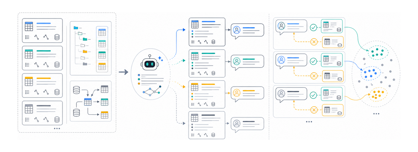
Fine-tuning an embedding model requires examples. It needs queries and the tables they should retrieve. It also needs negatives: tables that may look plausible but should not be returned for that query.

We did not have a mature production log of real user questions labelled with correct tables. Waiting for one would have been circular. Users need reliable retrieval before they can depend on the product, and we need usage before we can collect high-quality human labels. So we generated the training signal from metadata.

The first ingredient was a more consistent table representation. We already had Alation metadata across the catalogue, but search quality depends on consistency. A description written for a local data team is not always a good representation for an embedding model. We used Claude Sonnet via the corporate LLM gateway to generate bilingual English/Ukrainian descriptions from structural metadata, including table name, columns, types, layer, and lineage.

The prompt also produced category tags and a priority score. This mattered because not all tables should influence retrieval equally. A core transaction fact table should not be treated the same way as a temporary table, a vocabulary table, a technical mapping table, or an archive copy.

The second ingredient was synthetic user questions. For each table, Claude generated questions a real user might ask whose answer would require that table. Card tables received questions about card products and transactions. Customer tables received questions about entities and attributes. Fact tables received analytical questions. Around 20% of the generated output was not a full sentence but a short search phrase, because real users often type fragments like “card transaction volumes” or “залишки на рахунках” instead of complete questions.

The third ingredient was hard negatives. In contrastive training, a positive pair pulls the query and correct table closer together. A negative pair pushes the query and the wrong table apart. Random negatives are almost useless; the model does not need much help separating “card transactions” from an unrelated technical log table. The valuable examples are hard negatives: tables that share vocabulary and domain context but answer a different question.

This is the standard shape for embedding model training. Hands-On Large Language Models [5] describes contrastive learning as the mechanism that teaches an embedding space what should be close and what should be far apart, and it treats hard negatives as one of the most important levers in that process.

For example, a card-application table is a hard negative for “card purchase volume by merchant category.” Same domain vocabulary, different business object. A balance snapshot can be a hard negative for “transaction movements over time.” Same customer/account world, different measure. These are the distinctions the model needs to learn.

Hard negatives also create a bootstrapping problem. To find similar but incorrect tables, we need an embedding space. To get a good embedding space, we need robust hard negatives.

Our first bootstrap used a pre-trained multilingual E5-small model to build a temporary FAISS index over table descriptions. For each table, we retrieved nearby candidates. Then Claude classified each candidate as either positive, meaning genuinely related or valid for similar questions, or negative, meaning superficially similar but not answer-bearing for that intent.

Those labels became training data for BGE-M3. In one training generation, roughly 7K indexed tables produced about 430K training pairs. The live catalogue is larger and keeps changing, so the pipeline had to be repeatable. The generation cost was on the order of tens of dollars, which made retraining an engineering decision rather than a budget event.

At that point, the plan looked sound: better descriptions, bilingual questions, positives, hard negatives, and a strong multilingual base model.

Then the model started getting worse.

5. The improvement that made things worse

The first training run was intentionally limited. We trained on about 2K curated tables using hard negatives mined from the E5-small bootstrap index. It was not production-ready, but it gave us a useful baseline. A representative card-transaction table ranked 6th. Overall MAP@10 was 0.2741.

Then we scaled to the broader catalogue. Retrieval became harder, as expected. The same representative table fell to rank 15, and MAP@10 dropped to 0.1779. That was disappointing but understandable: more tables meant more competition.

For the next run, we tried ordinary tuning moves. We added category tags to the text and lowered the learning rate. The result got worse again. The representative transaction table moved to rank 16, and MAP@10 dropped to 0.1387.

Then we tried the improvement that should have helped most: iterative hard-negative mining. By this point, our own model had learned some structure in the banking domain. If hard negatives are nearby but wrong tables, our model should find better candidates than the generic E5-small bootstrap model. So we rebuilt the hard-negative lists using the v3 model’s embeddings and trained v4.

Aggregate MAP@10 rose from 0.1387 to 0.2021. If we had looked only at the aggregate, we might have called it progress.

But the transaction slice collapsed. The representative card-transaction table fell to rank 46, and other transaction tables showed the same pattern. Tables that should have appeared near the top for transaction questions were buried in the 30s, 40s, and 50s.

This was not one unlucky table. It was systematic. Several card-transaction tables from different databases should all have been near the top for broad questions like “show me card transactions.” But in reality, after training, they were drowned out together.

The benchmark exposed the symptom clearly. We had hundreds of synthetic queries that should have retrieved critical transaction fact tables. Instead, the model kept returning the same pool of similar-looking competitors. In one investigation, the target appeared only at rank 11 in its own query results; its hard negatives outranked it.

More training had not made the important tables more visible. It had made them less reachable.

6. Popular transaction tables were drowning each other out

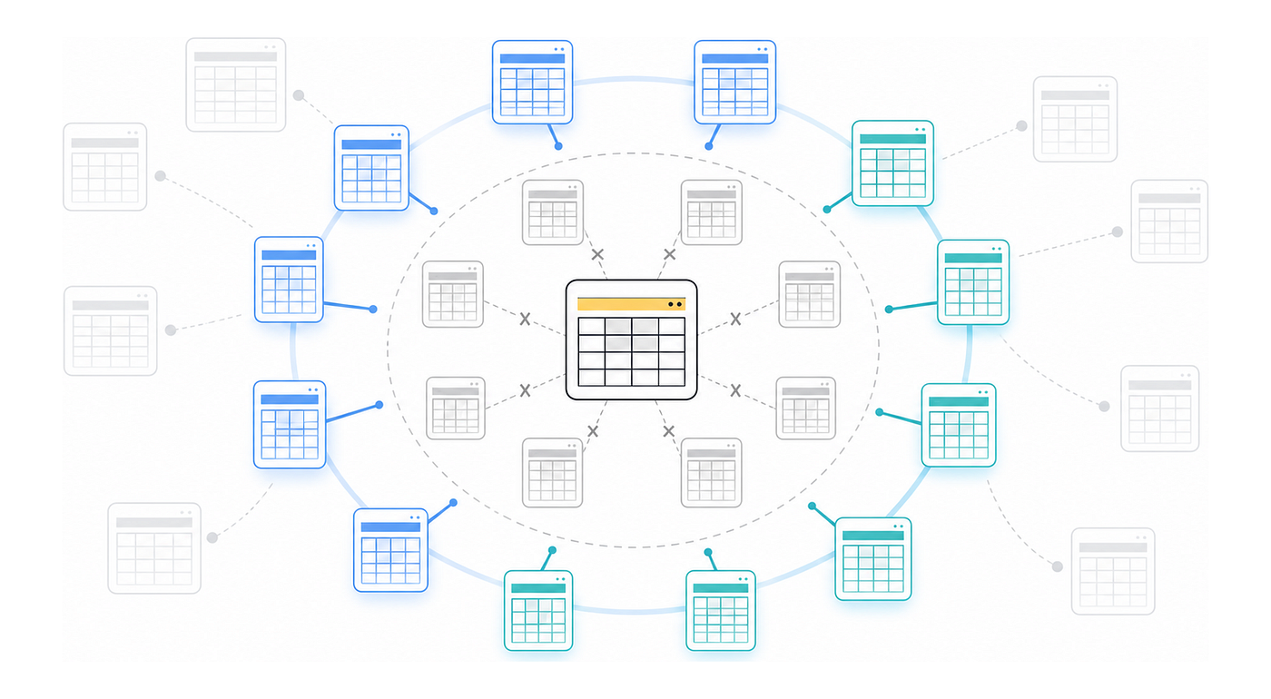
The Data Lake was not evenly distributed across topics. It had dense clusters: groups of tables that all described variations of the same business concept. Core banking data naturally forms these clusters. There are many transaction, balance, card, AML, risk, and application tables. Some come from different source systems. Some are curated views. Some are archive or SCD2 history versions. Some are daily aggregations over lower-grain facts.

These tables are not duplicates, but they share much of the same language. A transaction fact table, a transaction archive, a transaction-link table, a transaction vocabulary table, and a transaction-derived aggregate can all contain the words that a generic embedding model loves: transaction, amount, payment, card, currency, merchant, and account.

The important clusters looked roughly like this:

+----------------------------+----------------+--------------------------------------------+
| Cluster                    | Approx. tables | Shared vocabulary                          |
+----------------------------+----------------+--------------------------------------------+
| AML / financial monitoring | ~10            | entity, monitoring, suspicious, compliance |
| Accounts / balances / GL   | ~11            | account, balance, limit, currency          |
| Transactions / payments    | ~8             | transaction, amount, payment               |
| Risk / credit / DPD        | ~7             | default, DPD, credit, risk                 |
| Cards / loans              | ~5             | card, loan, application                    |
| Offers / CRM               | ~4             | customer, offer, client                    |
+----------------------------+----------------+--------------------------------------------+

In our internal priority scale, P5 refers to the most business-critical tables: core facts and entities that users are likely to ask for directly. Many P5 tables sit inside dense clusters because that is where the useful banking data lives. That is also where contrastive training became dangerous.

A positive pair pulls a query and a table together. A hard-negative pair pushes a query and a wrong table apart. In a sparse part of the catalogue, this works cleanly. If a query is about transactions, a remote technical log table is not nearby, and it does not matter.

Inside a dense cluster, the same rule can teach the model the wrong lesson. Imagine several transaction-related tables. They are close together because they genuinely share domain meaning, and for broad questions like “show me card transactions,” several of them should appear near the top. They may live in different databases or represent different stages of the transaction lifecycle, but they are all important answer-bearing candidates.

If those tables become hard negatives for each other, training pushes them apart. The model is not learning: “Put transaction facts above vocabulary tables.” It is learning “separate these transaction tables from one another.”

The most popular tables receive the most damage because they appear in many hard-negative lists. They are similar to many other tables, so they are selected often. They receive push from many directions, even when several of those neighbouring tables should remain close to transaction questions.

Meanwhile, lower-priority tables that share the same words can remain near the query region. Vocabularies, link tables, mappings, and secondary reference tables may be useful after the main fact tables, but they should not be first when the user asks for transactions. In our failed runs, they inherited positions that should have belonged to the transaction fact tables.

We started calling this failure mode mutual repulsion. Hard negatives were not bad in general; they were necessary. The problem was that our mining strategy selected the nearest neighbours inside dense clusters, and the nearest neighbours were often not safe negatives. Some were valid positives. Some were lineage siblings. Some were sibling facts from another source system. Some were different tables, but still part of the same answer-bearing family.

Iterative mining amplified the issue. The better the model became at recognising domain similarity, the more its nearest neighbours came from inside the same dense cluster. Then those neighbours became negative. Then the next model pushed the cluster apart harder.

The model was improving its picture of the domain and using that better picture to generate worse training data.

7. The fix was to stop trusting the closest neighbours

The fix was almost embarrassingly mechanical: when mining hard negatives, we stopped taking the closest neighbours.

Instead of using the nearest group of tables as candidates, we ignored the closest band and used the next band. Conceptually, we asked the index for a wider list, discarded the most similar cluster siblings, and sent the following candidates to Claude for classification.

After the fact, this looked less like a strange local trick and more like a known embedding-training pattern. Designing Large Language Model Applications [1] describes hard-negative margin mining in almost the same spirit: random negatives are too easy, but the nearest neighbours can be too hard or even false negatives, so a safer strategy is to mine from a middle band of candidates.

That sounds wrong until you remember what we needed. The closest tables were often siblings: related transaction tables, history tables, lineage-connected tables, or alternate valid sources. They shared most of the vocabulary and often represented useful answer-bearing data. They were exactly the tables most likely to create false negatives and mutual repulsion.

The next band of neighbours was different. Those tables still shared enough language to be confusing, but they were more likely to come from adjacent domains: risk tables mentioning limits and amounts, general-ledger tables mentioning currency and movements, card-master tables describing products rather than transactions. They were close enough to teach useful boundaries and far enough not to break the core cluster.

We spot-checked mined candidates at different skip levels:

+----------------------------+--------------------------+-----------------------+
| Nearest neighbours ignored | Genuinely hard negatives | False negatives       |
+----------------------------+--------------------------+-----------------------+
| 0                          | 55%                      | several               |
| 20                         | 50%                      | fewer                 |
| 50                         | 65%                      | 0 found in the sample |
+----------------------------+--------------------------+-----------------------+

Then we trained v5 from a fresh BGE-M3 checkpoint. We did not continue from v4 because we did not want to inherit its distorted neighbourhoods.

The result was the turning point. The representative card-transaction table recovered from rank 46 to rank 6. Its MAP@10 jumped from 0.034 to 0.474, and its Recall@10 rose from 20.2% to 82.1%. Aggregate MAP@10 in the targeted benchmark rose from 0.2021 to 0.4530.

The lesson is not “always ignore 50 neighbours.” That number belongs to our catalogue, model, and evaluation set. The lesson is more general: in a dense enterprise catalogue, the nearest neighbour is not automatically the best hard negative. Sometimes the nearest neighbour is a sibling, a duplicate, a lineage-connected table, or another valid answer. Treating it as a negative teaches the model a lie.

Hard negatives need distance from the positive, but not just any distance. They need to be close enough to be confusing and far enough not to be the same business concept.

8. The final model was not a one-trick

Skipping the closest neighbours rescued the model, but it did not finish the system. Later iterations were less dramatic and more practical. They made the training process respect the catalogue's shape rather than pretend that every table was equally important and equally distinct.

The first change was hybrid loss. Each training batch provides in-batch negatives: other examples’ positive tables. These are useful extra comparisons, but in our domain, some in-batch “negatives” are actually related tables. A query for one table may legitimately be answered by a lineage sibling. During training, we exclude known-positive related tables from the in-batch negative pool.

The second change was priority weighting. A P5 transaction fact table should affect the model more than a low-priority technical table. The base weight comes from detected priority, with extra weight for curated-layer and fact-category tables and reduced weight for duplicate-like or SCD2 tables.

The SCD2 reduction looks like a small implementation detail, but it encodes an important catalogue fact. Historical version tables often have near-identical descriptions to their parent tables. If they train with equal weight, they compete for the same top-K positions. Reducing their weight gives the canonical table a better chance to rank first while keeping the history table available when it is genuinely needed.

The third change was dynamic negative sampling. Each table can have many negative candidates. Instead of training on the same fixed subset every epoch, the loader samples a different subset during training. That reduces memorisation of individual negative pairs and makes the model learn a broader pattern.

The fourth change was per-priority evaluation. Aggregate MAP@10 was no longer enough. v4 had shown why: the aggregate can improve while critical tables collapse. P5 became a first-class quality slice, not a reporting detail hidden inside the mean.

Across eight iterations, the internal validation benchmark looked like this:

+---------+--------+-----------+------+-------------------------------------+
| Version | MAP@10 | Recall@10 | Rank | Change                              |
+---------+--------+-----------+------+-------------------------------------+
| v1      | 0.2741 | 70.3%     | 6    | Baseline, 2K tables                 |
| v2      | 0.1779 | 45.2%     | 15   | Scaled to broader catalogue         |
| v3      | 0.1387 | 41.3%     | 16   | Categories + lower learning rate    |
| v4      | 0.2021 | 54.2%     | 46   | Iterative mining failure            |
| v5      | 0.4530 | 86.5%     | 6    | Nearest-neighbour skip, fresh start |
| v6      | 0.5036 | 89.0%     | 6    | Dynamic negative sampling           |
| v7      | 0.4740 | 89.0%     | 6    | Conservative hyperparameters        |
| v8      | 0.5455 | 92.3%     | 3    | Priority + duplicate handling       |
+---------+--------+-----------+------+-------------------------------------+

Note: this table uses the internal validation benchmark we tracked while iterating on model versions. The OpenAI comparison earlier uses a smaller held-out test set, which is why the v8 values differ slightly.

The production model is v8. The exact decimals matter less than the shape of the curve. v4 looked mildly better in aggregate, but failed badly on critical transaction tables. v5 fixed the failure mode. v8 made the result stable enough to serve.

9. Production retrieval is a two-stage pipeline

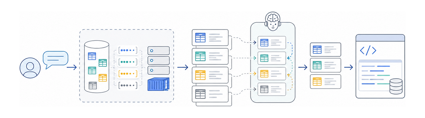
Once the model worked, production serving became a supporting part of the story rather than the story itself. The fine-tuned model runs behind a dedicated search service on AWS ECS Fargate. The main MCP server calls this service whenever the text-to-SQL agent needs table candidates: it sends the user question, receives ranked table results, and loads schemas for SQL generation.

The service has its own autoscaling logic. After each retraining run, we publish new model artefacts and point the ECS service to the new version through Terraform. The MCP server does not need to know how the model was trained; it depends on a stable table-search API.

There is one more layer after embedding retrieval. The MCP table-search tool receives two inputs: the user question and optional additional context. That context can include information from previous chat turns, related table names the agent has already found, or other clues collected during the task.

The embedding service performs a broad cut: from roughly 7K searchable tables to about 50 candidates worth looking at. The MCP server then asks Claude Sonnet to rerank that shortlist using the original question and the additional context, and passes only the ordered top 20 to the main agent. The result is not just a better ranking. It is a smaller, cleaner starting point for SQL generation, with less token waste and less work left for the agent.

This follows a common retrieval architecture. Hands-On Large Language Models [5] describes the bi-encoder versus cross-encoder split: a fast embedding model retrieves candidates, then a more expensive model reranks the shortlist. Our reranker fills the cross-encoder’s slot, but it is not a trained cross-encoder. It is Claude Sonnet doing listwise reranking. Instead of scoring each query-table pair separately, it reads the entire shortlist at once and can use the conversational context the agent has already gathered. The Machine Learning Solutions Architect Handbook [6] adds a second production reason for reranking: the best evidence must be selected and ordered before it enters the LLM’s context window.

This matters for quality and for systems design. With reranking, MAP@10 rises from about 0.59 for embedding retrieval alone to roughly 0.68–0.70. The main agent also receives a pre-sorted list reflecting the current conversation. It does not need to spend another LLM cycle deciding which table candidates look best, nor does it fill its context window with retrieval debate before SQL generation begins.

That separation of responsibilities made the pipeline easier to reason about. The embedding model is responsible for recall over the catalogue. The reranker is responsible for context-sensitive ordering among the top candidates. The SQL agent is responsible for using the selected schemas correctly.

When these responsibilities blur, debugging becomes vague. When they are separated, a bad answer becomes easier to inspect: did retrieval miss the right table, did reranking place it too low, or did SQL generation misuse the schema?

10. What I would take from this

The main lesson is not “fine-tune your embeddings.” Sometimes a generic embedding model is enough. Sometimes, a hybrid search or a reranker is the better investment. Sometimes the biggest problem in a text-to-SQL system is not retrieval at all but schema rendering, SQL validation, permissions, or user trust.

The lesson is narrower and more useful: if your RAG target is not actually text, do not assume that text-similarity embeddings solve the right problem.

Our target was a data asset. The user’s question was not looking for a paragraph with similar wording. It was looking for the place in the data model where the answer could be computed. That changed the training data, the evaluation, the failure modes, and the fixes.

Four practical points follow from that.

First, evaluate the retrieval decision your product actually depends on. For us, Recall@10 mattered because the LLM needed the correct table inside the candidate set. A nice semantic-search demo means little if the answer-bearing table is absent.

Second, hard negatives are not automatically good because they are near. In dense enterprise catalogues, nearest neighbours are often siblings, duplicates, lineage-connected tables, or alternate valid answers. Push them apart blindly, and you can bury your best tables.

Third, aggregate metrics hide the failures users will notice. v4 looked mildly better in aggregate and catastrophically worse for important transaction tables. Per-priority metrics were not a reporting nicety. They were a debugging tool.

Fourth, single-label evaluation has a ceiling in data systems. If several lineage-connected tables can answer the same business question, a metric that marks only one as correct will punish useful retrieval. We still need better cluster-aware evaluation that treats equivalent answer-bearing tables as valid.

The model did not make the entire LLM agent trustworthy on its own. The LLM can still write the wrong SQL against the right tables. The schema context can still be too large. Validators can reject useful queries. Users still need to learn where the agent is reliable and where it is not.

What the model changed was narrower and more important: it made the right tables visible often enough for the rest of the system to matter. Before fine-tuning, the agent saw the right table in the top 10 about half the time. After fine-tuning, it saw it nearly nine times out of ten. Reranking improved the final ordering further.

That does not settle product adoption. It does not prove users' trust in every answer. It does not remove the need for supervision.

But it turns text-to-SQL over the Data Lake from impossible into possible.

Further reading

[1] Designing Large Language Model Applications (Suhas Pai, 2025): long-context tradeoffs, production RAG stages, and hard-negative margin mining.

[2] Agentic Design Patterns (Antonio Gullí, 2025): context engineering as the discipline of selecting and packaging the right information for each LLM step.

[3] Modern Data Architecture on AWS (Behram Irani, 2023): natural-language-to-SQL patterns grounded by catalogue metadata.

[4] AI Engineering: Building Applications with Foundation Models (Chip Huyen, 2025): retrieve-then-generate architecture and the importance of evaluating retrievers independently.

[5] Hands-On Large Language Models (Jay Alammar and Maarten Grootendorst, 2024): contrastive learning, hard negatives, and the bi-encoder / cross-encoder retrieval split.

[6] The Machine Learning Solutions Architect Handbook, Second Edition (David Ping, 2024): reranking, context ordering, and the lost-in-the-middle problem in production RAG.

[7] Architecting Data and Machine Learning Platforms (Marco Tranquillin, Valliappa Lakshmanan, and Firat Tekiner, 2023): the data catalogue as a first-class discoverability layer.

[8] Data Quality Fundamentals (Barr Moses, Lior Gavish, and Molly Vorwerck, 2022): data discovery versus static cataloguing in lake-scale and distributed data platforms.