How Jerzy Neyman Changed Sampling Forever

Why the intuitive idea of the “miniature population” failed, and what replaced it

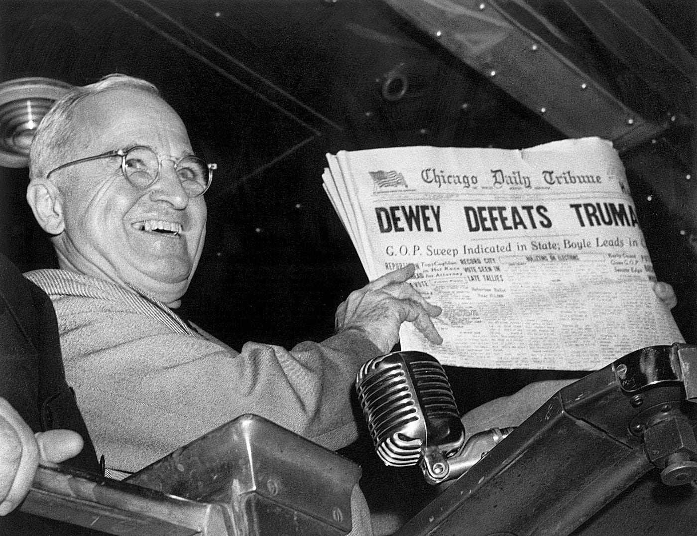
Fig 1: Harry Truman triumphantly holds the erroneous “Dewey Defeats Truman“ headline, November 1948. (Image courtesy of Wikimedia Commons)

In 1948, Harry Truman held up a newspaper bearing one of the most famous mistaken headlines in history: “Dewey Defeats Truman.”

The photograph became a lasting symbol of polling failure. But the deeper story began fourteen years earlier, in a lecture hall in London, when the Polish mathematician Jerzy Neyman (1894–1981) challenged one of the most intuitive ideas in statistics:

A good sample should look like a small-scale copy of the population.

It sounds obvious. It feels sensible. If the population is 50% female, 30% rural, and 20% wealthy, then surely the sample should have those same proportions too.

For a long time, that was exactly how many people thought about representativeness. But Neyman showed why this intuition could be badly misleading.

His 1934 paper did more than refine a technical method. It changed what statisticians believed a sample was for.

The Seductive Idea of the “Miniature Population”

By the 1920s, statisticians had already accepted an important idea: you do not always need a full census to learn about a population. A properly chosen sample could be enough (see previous article).

But that raised a harder question:

If you are not going to count everyone, how should you choose the few who speak for the many?

For years, two rival answers coexisted uneasily:

• random selection, grounded in probability;
• purposive selection, grounded in expert judgement.

Purposive sampling had enormous appeal. Its logic was simple and visually convincing. If the population contains certain proportions of men and women, urban and rural residents, rich and poor, then the sample should reproduce those proportions. Build a balanced miniature, and it should reveal the truth about the whole.

This way of thinking felt scientific. It also felt safer than randomness.

After all, random sampling can look untidy. What if chance produces too many rich respondents? What if it misses an important subgroup? What if the sample simply does not look representative?

Even Arthur Bowley (1869–1957), a leading advocate of random sampling, favoured proportional allocation within stratified designs (i.e. sampling strata strictly according to their sizes in the population). Beneath that preference lay a powerful assumption:

Representativeness meant resemblance.

Neyman’s great insight was that this confused appearance with validity.

Neyman’s 1934 Challenge

Fig 2: Jerzy Neyman (left, image courtesy of The University of York) and Arthur Bowley (right, image courtesy of Wikimedia Commons) represented two different ideas of what a “representative” sample should be.

In 1934, Neyman, then aged 40, presented a landmark paper to the Royal Statistical Society: “On the two different aspects of the representative method: the method of stratified sampling and the method of purposive selection”.

What made the paper so powerful was that Neyman did not rely on theory alone. He tested the issue against real data.

A few years earlier, the Italian statisticians Corrado Gini (who developed the Gini coefficient, a measure of the income inequality in a society) and Luigi Galvani had faced an unusual problem. Before the paper records of the 1921 Italian census were destroyed, they were asked to preserve a sample of them. They selected 29 out of 214 administrative districts using purposive methods.

Because the full census values were known, Neyman had a rare opportunity: he could compare the sample directly with reality.

Gini and Galvani had carefully chosen districts so that the sample matched national averages on seven important control variables, including birth rates, death rates, marriage rates, mean income, the share of the male agricultural population, urbanisation, and altitude.

On paper, the sample looked excellent. It resembled the population on precisely the characteristics its designers had targeted.

But when Neyman examined variables outside those controls, the picture changed. The sample diverged sharply from the full population. By choosing districts close to the national averages, the designers had unintentionally removed much of the natural variation that actually existed in Italy. The sample looked balanced, but it was too smooth, too centred, too tidy. It failed to capture the real spread of the population and distorted the relationships among variables.

That was Neyman’s point.

A sample can resemble the population and still mislead you.

Matching a few visible characteristics does not guarantee accuracy on everything else. A purposive sample may look representative while failing on the very quantities you care about.

This was not a minor correction. It was a direct challenge to the intellectual foundation of purposive selection.

The Deeper Break: Sampling is about Uncertainty, not Visual Balance

Neyman’s critique did not stop with purposive sampling. He also showed that strictly proportional allocation in stratified random sampling is not generally the most efficient design.

Suppose a population is divided into strata, and some strata are much more variable than others. In that case, sampling each stratum in exact proportion to its size is often wasteful. A large but internally homogeneous group may require relatively few observations. A smaller but more variable group may require many more.

In other words, if your goal is precision, a good sample will often not look like a miniature of the population.

This was a profound shift.

The purpose of a sample is not to imitate the population visually. It is to support inference while minimising uncertainty.

That idea is now so familiar that it can be hard to appreciate how radical it once sounded.

Bowley and the Older Intuition

Arthur Bowley, then aged 65, was in the audience when Neyman presented his paper. By then, Bowley was one of the most respected figures in British statistics and a major architect of random sampling in social research.

He expressed reservations about Neyman’s departure from strictly proportional sampling and famously characterised Neyman’s newly introduced concept of “confidence intervals” as a “confidence trick”. Another giant of statistics in the audience, R.A. Fisher, raised a practical objection to Neyman’s optimal allocation: If different strata should be sampled at different rates because they have different variances, Fisher asked, how can one possibly know those variances before conducting the survey?

While Neyman did not fully resolve Fisher’s logistical challenge in his reply, the practical answer soon became a cornerstone of modern survey design: exact knowledge is not necessary. Approximate information from previous studies, administrative records, or small pilot surveys is often enough to estimate these variances and improve the design substantially. One does not need perfect foresight to do better than blindly assuming every group should be sampled in strict proportion to size.

That exchange captured a turning point. Bowley represented an older intuition: that balance and proportion were central to representativeness. Neyman represented a newer one: probability-based design exists to control error, not to produce a pleasing miniature.

The transition was not instantaneous, but the centre of gravity had shifted.

(See Appendix for a mathematical proof why Neyman allocation outperforms proportional allocation.)

Pollsters Learnt the Lesson the Hard Way

While academia accepted Neyman’s mathematical proof relatively quickly, the commercial polling world learnt the lesson more painfully.

In the 1936 U.S. presidential election, The Literary Digest conducted an enormous poll and predicted that Alf Landon would defeat Franklin D. Roosevelt. Its sample was huge: millions were contacted, and about 2.4 million responses were returned. But it was drawn from car registrations and telephone directories, which overrepresented more affluent Americans during the Great Depression.

The result was a disaster.

Fig 3: (Left) A cover of The Literary Digest. (Wikimedia Commons) (Right) Americans enjoying an outing by car in the 1930s; car registration lists helped produce a wealth-biased sampling frame. (Wikimedia Commons)

At the same time, George Gallup used a much smaller quota-style sample (about 50,000 people) and correctly predicted Roosevelt’s victory. For a moment, this seemed like a triumph for the “miniature population” idea. If a carefully balanced sample could beat a gigantic but biased one, maybe purposive selection really was the answer.

But quota sampling had a hidden weakness. Even when quotas were carefully specified: find 5 urban men under 40, 3 rural women over 40, and so on, interviewers still had discretion over which individuals they approached within each category. That final step was not random.

The weakness of quota sampling became impossible to ignore in 1948, when major pollsters predicted that Thomas Dewey would defeat Harry Truman. Interviewers tended to select respondents who were easier to reach or more willing to talk, allowing hidden biases to creep in. The error was also worsened because many polls stopped interviewing too early and missed late movement toward Truman.

The result was the most famous polling embarrassment in American history.

After 1948, confidence in quota methods weakened sharply, and probability-based sampling gradually became the standard for serious survey inference.

Neyman’s warning had become public reality.

Why Neyman Allocation Mattered

The principle that emerged from this debate is now often called Neyman allocation.

Its intuition is simple. Imagine a population composed of two groups:

• a large group whose values are relatively stable;
• a smaller group whose values vary enormously.

If your goal is to estimate the population average as precisely as possible under a given sample size, it makes little sense to sample strictly in proportion to group size. The more variable group contributes more uncertainty, so it deserves more sampling effort. The more stable group contributes less uncertainty, so it can be sampled more lightly.

Fig 4: The idea behind Neyman Allocation (Image by author)

That means the most statistically efficient sample may look less like the population in raw proportions — and yet produce better inference.

This is the conceptual break Neyman forced statisticians to make:

Representativeness is not the same as proportional resemblance.

Once that becomes clear, the “miniature population” ideal starts to collapse.

Why This Still Matters in the Age of AI

Neyman’s logic also feels surprisingly modern.

Consider a fraud-detection model. In the real world, fraudulent transactions may account for only a tiny fraction of all cases. If you train a model on data that mirrors those proportions too closely, the model can achieve excellent headline accuracy simply by predicting the majority class almost all the time — while failing at the task you actually care about.

That is why machine-learning practitioners often oversample minority cases, undersample majority cases, or use other methods designed for imbalanced data. The training data are deliberately adjusted so the model pays attention to rare but important patterns.

Fig 5: An illustration of an imbalanced dataset (Image by author)

This is not the same thing as Neyman allocation in a strict survey-sampling sense. The goals are different, and the mathematics is not identical.

But the intellectual resemblance is striking:

A useful sample for learning does not always need to mirror the world in simple proportion.

In both cases, the deeper principle is the same. The right sample depends on the purpose. Sometimes proportional resemblance helps. Sometimes it hurts.

The End of the Miniature

Today, whether in official statistics, survey research, polling, or data science, we still live with Neyman’s central insight.

Human judgement still matters. It matters when defining populations, building sampling frames, designing strata, writing questions, and handling nonresponse. But judgement alone cannot justify inference if you want uncertainty that can be measured.

That is what probability sampling changed.

Randomisation does not guarantee a perfect sample. What it provides is something more important: a principled way to quantify error and make defensible statements about a population.

That was Neyman’s lasting break with the old ideal of the miniature population.

A sample does not become valid because it looks balanced.

It becomes valid because its uncertainty can be understood.

👉 Read the Chinese version **here**

References

1. He, H., & Garcia, E. A. (2009). “Learning from Imbalanced Data.” IEEE Transactions on Knowledge and Data Engineering, 21(9), 1263–1284.
2. Mosteller, F., Hyman, H., McCarthy, P. J., Marks, E. S., & Truman, D. B. (1949). “The Pre-Election Polls of 1948: Report to the Committee on Analysis of Pre-Election Polls and Forecasts.” Social Science Research Council, Bulletin 60.
3. Neyman, J. (1934). “On the two different aspects of the representative method: the method of stratified sampling and the method of purposive selection.” Journal of the Royal Statistical Society, 97(4), 558–625.
4. Squire, P. (1988). “Why the 1936 Literary Digest Poll Failed.” Public Opinion Quarterly, 52(1), 125–133.