ZK: How a Halo2 Fibonacci Circuit Translates to Polynomials

Contents

1. Introduction
2. Halo2 Circuits 2.1 Advice and Instance Columns 2.2 Gates, Constraints, Selectors 2.3 Chips, Regions, Layouter
3. Fibonacci Circuit Code
4. Fibonacci Circuit Layout 4.1 Pallas Curve 4.2 Synthesizing the Circuit 4.3 Copy Constraint
5. Calculating the Circuit Polynomials 5.1 Primitive nth Roots of Unity 5.2 Interpolation via Inverse Fast Fourier Transform 5.3 Advice, Selector, Constraint, Vanishing, Quotient Polynomials 5.4 Fibonacci Circuit Polynomials Script 5.5 Calculated Coefficients Using IFFT
6. Conclusion
7. References

1.0 Introduction

Zero-Knowledge Proof Systems (ZKPS) require efficient encoding of circuits into mathematical structures. This translation enables succinct proof verification. Halo2, a PLONKish SNARK, achieves this through polynomial interpolation. Major parts of the circuit (constraints, advice values, selectors, etc.) are encoded as polynomials over a finite field.

This article examines how a Fibonacci sequence Halo2 circuit is translated from the high-level Halo2 API to low-level math. The Halo2 API code is provided and decomposed into the advice, selector, constraint, vanishing, and quotient polynomials. The key insight, checking all constraints in O(1) operations via polynomial remainder theorem and Schwartz-Zippel Lemma, is explained. This article does not formally cover Halo2’s Polynomial Commitment Scheme (KZG), or the complete PLONK process. That said, understanding the translation from circuits to polynomials is foundational to understanding Halo2. Additionally, although the Fibonacci circuit is simple, it implements many core concepts from the Halo2 API.

2.0 Halo2 Circuits

Halo2 circuits involve the evaluation of gates and constraints. In these circuits, columns are different variables, and rows are iterations of the computation. The columns, rows, gates, constraints, selectors etc. of the circuit make up the layout. This section will explain the concepts involved with Halo2 circuits/the Halo2 API, provide code for a Fibonacci Sequence circuit, and show relevant logging output.

2.1 Advice and Instance Columns

As previously stated, columns of a Halo2 circuit represent variables. As variables change throughout the circuit’s computations, their values are recorded in the rows of the layout. This means that a cell holds the value of a variable at a given iteration. For this simple Fibonacci circuit, two types of columns are used: advice columns, and instance columns. Advice columns hold private and intermediate values, which are not publicly exposed. Thus, the advice column(s) are part of the witness. Instance columns, on the other hand, are exposed to the public and thus not part of the witness. Halo2 supports other column types, e.g. fixed columns, but for the Fibonacci Sequence, they are not needed.

2.2 Gates, Constraints, Selectors

In Halo2, operations on variables, within the circuit, are done with gates. Gates are evaluated using a constraint, or a computation that is evaluated against 0. The constraint for the fibonacci_add gate is vec![s_add * (prev + curr — next)]. If this computation equals 0, the constraint is met. Conversely, if the result is nonzero, an error has occurred. The Rotation structure implements methods to “rotate” over a column’s values. This rotation is explained mathematically in section 5.3.

Since this Fibonacci Circuit only uses one advice column, each element of the sequence is stored in a different row. Thus, the next value of the sequence is equal to the sum of the current and previous advice column cells. If the constraint s_add * (prev + curr — next) = 0 the Fibonacci Sequence is correctly followed since next = prev + curr. The s_add variable is a selector, with a value of 1 or 0. The selector determines whether the gate is active for a given row. If the selector is enabled (value 1) then the gate and constraint are computed, otherwise the gate is not enabled. If the gate is not enabled, then the constraint automatically evaluates to 0 since s_add = 0 . Below is the code needed to create this gate using the Halo2 crate halo2_proofs .

 meta.create_gate(
    "fibonacci add", |meta| {
    let prev = meta.query_advice(advice, Rotation::prev());
    let curr = meta.query_advice(advice, Rotation::cur());
    let next = meta.query_advice(advice, Rotation::next());
    let s_add = meta.query_selector(s_add);
    vec![s_add * (prev + curr - next)]
});

2.3 Chips, Regions, Layouter

In Halo2, chips are used to create modular circuits. Chips in the circuit enable modular designs because chips are reusable, and abstractly defined. The chip has a set of gates that it is configured to use, thus providing a layer of abstraction above individual gates and constraints¹. With complicated, or long circuits, many chips may be needed. For this simple Fibonacci circuit, however, only one chip is used. In addition to the needed gates and constraints, the chip is configured with the necessary columns. When a chip is synthesized, the cell values are computed, and the appropriate instance values are exposed.

Regions are Halo2’s way of dividing a circuit. More specifically, each region is a disjoint subset of cells in the circuit¹. Relative references are specific to the region in question, so row 0 in region A is not the same as row 0 in region B. The Layouter is Halo2’s organizer. It is responsible for enabling selectors, assigning values to cells, managing region boundaries and more.

3.0 Fibonacci Circuit Code

use std::marker::PhantomData;
use ff::Field;
use halo2_proofs::{
    circuit::{AssignedCell, Chip, Layouter, SimpleFloorPlanner, Value},
    plonk::{Advice, Circuit, Column, ConstraintSystem, Error, Instance, Selector},
    poly::Rotation,
};

// structure for the configuration for the chip
#[derive(Clone, Debug)]
struct FibChipConfig {
    advice: Column<Advice>, // 1 advice column to store 1 value of the sequence per row
    instance: Column<Instance>, // one instance column to store the sum of the previous 2 values in the sequence
    s_add: Selector,
}

// structure for the chip we need
struct FibChip<F: Field> {
    config: FibChipConfig,
    _marker: PhantomData<F>,
}

// structure to store numbers in cells
#[derive(Clone)]
struct Number<F: Field>(AssignedCell<F, F>);

// structure for the circuit
#[derive(Default, Clone)]
struct FibCircuit<F: Field> {
    a: Value<F>,
    b: Value<F>,
    num_steps: usize,
}

// implementing the Chip trait for FibChip
impl<F: Field> Chip<F> for FibChip<F> {
    type Config = FibChipConfig;
    type Loaded = ();

    // getter for the FibChipConfig of this FibChip instance
    fn config(&self) -> &Self::Config {
        &self.config 
    }

    // getter for the loaded field
    fn loaded(&self) -> &Self::Loaded {
        &()
    }
}

trait NumericInstructions<F: Field>: Chip<F> {
    type Num;

    fn expose_as_public(&self, layouter: impl Layouter<F>, num: Self::Num, row: usize) -> Result<(), Error>;
    fn fibonacci_sequence(
        &self, 
        layouter: impl Layouter<F>, 
        a: Value<F>, 
        b: Value<F>,
        num_steps: usize
    ) -> Result<Self::Num, Error>;
}

impl<F: Field> FibChip<F> {
    fn construct(config: <Self as Chip<F>>::Config) -> Self {
        FibChip { config, _marker: PhantomData, }
    }

    fn configure(
        meta: &mut ConstraintSystem<F>,
        advice: Column<Advice>,
        instance: Column<Instance>,
    ) -> <Self as Chip<F>>::Config {
        meta.enable_equality(instance);
        meta.enable_equality(advice);
        let s_add = meta.selector();

        meta.create_gate(
            "fibonacci add", |meta| {
                let prev = meta.query_advice(advice, Rotation::prev());
                let curr = meta.query_advice(advice, Rotation::cur());
                let next = meta.query_advice(advice, Rotation::next());
                let s_add = meta.query_selector(s_add);
                vec![s_add * (prev + curr - next)]
            });

        FibChipConfig {
            advice, 
            instance,
            s_add,
        }
    }
}

impl<F: Field> NumericInstructions<F> for FibChip<F> {
    type Num = Number<F>;

    fn expose_as_public(&self, mut layouter: impl Layouter<F>, num: Self::Num, row: usize) -> Result<(), Error> {
        let config = self.config();
        layouter.constrain_instance(num.0.cell(), config.instance, row)
    }

    fn fibonacci_sequence(
        &self, 
        mut layouter: impl Layouter<F>, 
        a: Value<F>, 
        b: Value<F>,
        num_steps: usize
        ) -> Result<Self::Num, Error> {
        let config = self.config();
        layouter.assign_region(
            || "fibonacci sequence", |mut region| {
                let mut prev_cell = region.assign_advice(
                    || "f_{i-1}", 
                    config.advice, 
                    0, 
                    || a
                )?;

                let mut curr_cell = region.assign_advice(
                    || "f_i", 
                    config.advice, 
                    1, 
                    || b
                )?;

                for i in 2..num_steps {
                    config.s_add.enable(&mut region, i-1)?;
                    let next_value = prev_cell.value().copied() + curr_cell.value().copied();
                    println!("Row {}: prev={:?}, curr={:?}, next={:?}", i, prev_cell.value(), curr_cell.value(), next_value);
                    let next_cell = region.assign_advice(
                        || "f_{i+1}",
                        config.advice,
                        i,
                        || next_value,
                    )?;

                    prev_cell = curr_cell;
                    curr_cell = next_cell;
                }

                Ok(Number(curr_cell))
            }
        )
    }
}

impl<F: Field> Circuit<F> for FibCircuit<F> {
    type Config = FibChipConfig;
    type FloorPlanner = SimpleFloorPlanner;

    fn without_witnesses(&self) -> Self {
        Self::default()
    }

    fn configure(meta: &mut ConstraintSystem<F>) -> Self::Config {
        let advice = meta.advice_column();
        let instance = meta.instance_column();
        FibChip::configure(meta, advice, instance)
    }

    fn synthesize(&self, config: Self::Config, mut layouter: impl Layouter<F>) -> Result<(), Error> {
        let chip = FibChip::construct(config);
        let result = chip.fibonacci_sequence(
            layouter.namespace(|| "fib sequence"), 
            self.a, 
            self.b, 
            self.num_steps
        )?;

        let _ = chip.expose_as_public(layouter.namespace(|| " result"), result, 0);

        Ok(())
    }
}

// main function
fn main() {
    use halo2_proofs::{dev::MockProver, pasta::Fp};
    println!("[*] Starting Halo2 Fibonacci Circuit");

    let k = 4; 
    let a = Fp::from(1);
    let b = Fp::from(1); // the Fibonacci sequence starts at 1, 1
    let num_steps = 10;

    let circuit = FibCircuit {
        a: Value::known(a), 
        b: Value::known(b), 
        num_steps,
    };

    let expected = vec![Fp::from(55)];
    let prover = MockProver::run(k, &circuit, vec![expected]).unwrap();
    assert_eq!(prover.verify(), Ok(()));
}

The code uses the Halo2 API crate to provide traits to implement and types. The documentation for this crate can be found in the references section. The MockProver is provided by Halo2 as a way to test circuits. It simulates the generation of a proof, and verification.

Running the code produces logging output shown below:

Row 2: prev=Value { inner: Some(0x1) }, curr=Value { inner: Some(0x1) }, next=Value { inner: Some(0x2) }
Row 3: prev=Value { inner: Some(0x1) }, curr=Value { inner: Some(0x2) }, next=Value { inner: Some(0x3) }
Row 4: prev=Value { inner: Some(0x2) }, curr=Value { inner: Some(0x3) }, next=Value { inner: Some(0x5) }
Row 5: prev=Value { inner: Some(0x3) }, curr=Value { inner: Some(0x5) }, next=Value { inner: Some(0x8) }
Row 6: prev=Value { inner: Some(0x5) }, curr=Value { inner: Some(0x8) }, next=Value { inner: Some(0xd) }
Row 7: prev=Value { inner: Some(0x8) }, curr=Value { inner: Some(0xd) }, next=Value { inner: Some(0x15) }
Row 8: prev=Value { inner: Some(0xd) }, curr=Value { inner: Some(0x15) }, next=Value { inner: Some(0x22) }
Row 9: prev=Value { inner: Some(0x15) }, curr=Value { inner: Some(0x22) }, next=Value { inner: Some(0x37) }

4.0 Fibonacci Circuit Layout

The FibCircuit structure has fields for the sequence starting points, and a number of iterations. The circuit only needs to run for a finite number of iterations, because circuits are used to compute witness and instance data for a specific output. In this case, the desired output is 55. This section dives into how the selectors are enabled, how the cells get populated, and the process involved with exposing the instance value(s).

4.1 Pallas Curve

Since the circuit operations are all over a finite field, we need a type that implements the Field trait. For this simple circuit we are using the Pallas base field². This curve is defined by the modulus 0x40000000000000000000000000000000224698fc094cf91b992d30ed00000001. There are other options for finite fields, with different properties for Halo2, but the Pallas Curve suffices for the Fibonacci Circuit.

4.2 Synthesizing the Circuit

Once all the configurations for the circuit are defined, the circuit can be synthesized. This is the process of computing witness values, exposing instance values, and preparing for constraint evaluation. In Halo2 the selector for row i is enabled at iteration i+1 meaning:

• Row 0: contains the first starting value (1). The selector is off (0) since there is no previous row to check.
• Row 1: contains the second starting value (1). The selector is on (1), but enabled when calculating the value in row 2.
• Row 2: contains the sum of the previous two values (2). The selector at row 1 is enabled, checking that 1+1–2 = 0.

This process repeats until the last used row, which has its selector off (0), and contains the last sequence value (55). The computation stops at this row because the predefined number of iterations has been completed. The last value (55) is bound by the copy constraint to the instance column, as detailed in the next section.

4.3 Copy Constraint

Once the appropriate number of Fibonacci iterations has been completed, the target cell needs to be exposed. To do this the Layouter enforces a copy constraint between the target cell in the advice column, and an instance column cell. The copy constraint enforces equality between the two cells, making it conceptually and mathematically different from gate constraints.

• Advice[9] = 55 <— —COPY — — > Instance[0] = 55
• Instance[0] exposed

5.0 Calculating the Circuit Polynomials

As previously mentioned, Halo2 (and other SNARKs) encode circuits as polynomials to enable a PCS. Using a PCS (Halo2 uses KZG) allows for succinct representation, efficient verification of computations, and more. This section details how the Fibonacci circuit shown is translated into polynomials. Importantly, because Halo2 uses the Inverse Fast Fourier Transform (IFFT) for polynomial interpolation, the k parameter must be a power of 2. This is detailed more in this section.

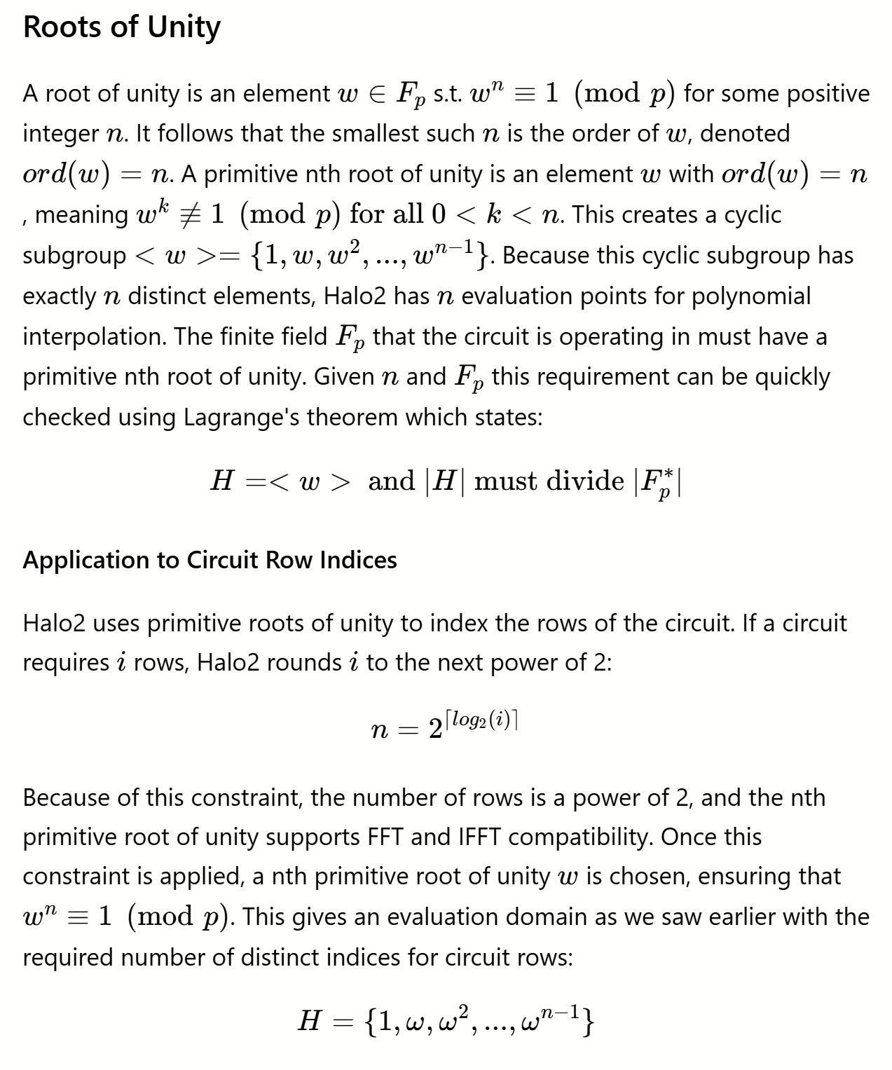
5.1 Primitive nth Roots of Unity

Below is a summary of what roots of unity are, and why they are needed for Halo2 polynomial interpolation.

5.2 Interpolation via Inverse Fast Fourier Transform

Polynomial Interpolation, in the context of Halo2, is performed via a Radix-2 Inverse Fast Fourier Transform (IFFT). The FFT and IFFT allow mapping between the evaluation domain and polynomial coefficients, as this section explains³.

Given the layout from section 3, after synthesis, the vector representing the advice column is: [0x1, 0x1, 0x2, 0x3, 0x5, 0x8, 0xd, 0x15, 0x22, 0x37, 0, 0, 0, 0, 0, 0]. The cell holding the value 0x37 from the advice column is copied to the instance column, and publicly exposed. The selector column vector is: [0, 1, 1, 1, 1, 1, 1, 1, 1, 0, 0, 0, 0, 0, 0, 0]. Even though only 10 rows are used to compute num_steps iterations, the circuit is padded to the next power of 2, enabling FFT/IFFT as previously discussed.

5.3 Advice, Selector, Constraint, Vanishing, Quotient Polynomials

The coefficients of the advice and selector polynomials are computed using the IFFT as seen in the previous section. The constraint, vanishing, and quotient polynomials require additional steps. This section explains why each polynomial is needed, and how Halo2 calculates it.

The vanishing polynomial provides an efficient method for verifying the constraints across the entire evaluation domain. Without the vanishing polynomial, the constraint polynomial would need to be evaluated at each row index, which is much less efficient than the computations below⁵

5.4 Fibonacci Circuit Polynomials Script

This section presents a Python script to compute the advice and selector polynomials. It takes a primitive nth root of unity and uses that to compute the evaluation domain. Then the script uses a simple IFFT implementation to calculate coefficients.

from Crypto.Util.number import inverse

# find a primitive nth root of unity mod p
def find_root_of_unity(n, p):
    g = 5 # known generator 
    omega = pow(g, (p-1) // n, p) # keep this simple for example sake
    assert pow(omega, n, p) == 1

    return omega

# simple inverse fast fourier transform calculations
def quick_ifft(eval_domain, values, n, omega, p):
    coefficients = []
    n_inv = inverse(n, p)
    omega_inv = inverse(omega, p)

    # outer loop for all the coefficients needed
    for k in range(n):
        c_k = 0
        omega_power = 1
        omega_step = pow(omega_inv, k, p)
        # inner loop for the summation
        for j in range(n):
            c_k = (c_k + values[j] * omega_power) % p
            omega_power = (omega_power * omega_step) % p

        # multiply by 1/n 
        c_k = (c_k * n_inv) % p
        coefficients.append(c_k)

    return coefficients

# given X as input and polynomial coefficients, compute output and return result
def evaluate_polynomial(X, coefficients, p):
    result = 0
    x_power = 1 # start from x^0 = 1

    # the degree of the terms goes up each iteration
    for c in coefficients:
        result = (result + c * x_power) % p
        x_power = (x_power * X) % p

    return result

# verify that the polynomial generated yields the correct value given omega^i
def verify(coefficients, omega, n, values, p):
    assert len(coefficients) == n
    # verify coefficients by checking A(X) = a_i for the advice values
    for i in range(len(values)):
        X = pow(omega, i, p) # A(omega^i) = a_i is the condition to check
        result = evaluate_polynomial(X, coefficients, p)
        assert result == values[i]
        print(f"[*] Success, f(X) = f_i for sequence value: {values[i]}")

# main function
def main():
    # Pallas Base Field prime
    p = 0x40000000000000000000000000000000224698fc094cf91b992d30ed00000001
    # define n based on the k parameter
    k = 4
    n = 2**k
    # column values
    advice_values = [1, 1, 2, 3, 5, 8, 13, 21, 34, 55, 0, 0, 0, 0, 0, 0]
    selector_values = [0, 1, 1, 1, 1, 1, 1, 1, 1, 0, 0, 0, 0, 0, 0, 0]

    # find the coefficients
    omega = find_root_of_unity(n, p)
    omega_inv = inverse(omega, p)
    print(f"[*] Using {n}th root of unity: {omega}")
    eval_domain = [pow(omega, i, p) for i in range(n)]
    advice_coefficients = quick_ifft(eval_domain, advice_values, n, omega, p)
    verify(advice_coefficients, omega, n, advice_values, p)

    # calculate the selector polynomial 
    selector_coefficients = quick_ifft(eval_domain, selector_values, n, omega, p)
    print(selector_coefficients)
    verify(selector_coefficients, omega, n, selector_values, p)

    # calculate the constraint polynomial and verify it vanishes
    for i in range(n):
        x = pow(omega, i, p)
        x_prev = (omega_inv * x) % p
        x_curr = x
        x_next = (omega * x) % p

        a_prev = evaluate_polynomial(x_prev, advice_coefficients, p)
        a_curr = evaluate_polynomial(x_curr, advice_coefficients, p)
        a_next = evaluate_polynomial(x_next, advice_coefficients, p)
        s_curr = evaluate_polynomial(x_curr, selector_coefficients, p)

        temp = (a_prev + a_curr - a_next) % p
        assert (s_curr*temp) % p == 0

        print(f"[*] Constraint polynomial vanishes on row: {i}")

if __name__ == '__main__':
    main()

5.5 Calculated Coefficients Using IFFT

The coefficients calculated for the advice and selector polynomials, are listed below:

# coefficients for the advice polynomial A(X)
[1809251394333065553493296640760748560210191030121347544747167297771872976905, 
2121961144179437140289205723028731038872226056984153478422336376911203473159, 
11531646231706255814986641157874235662294584338834212741923075038550015906728, 
9069568115408854334251815944776449183247933653828895032739713351518737193290, 
23134217551993789458220032207545177402210708370531564930895291928331419498209,
21682919351681383962706725061114709617393582357057927770824223764975977463541, 
1155480918279543228106331494165194578585681098474957216714640186142762344048, 
4442962637088384183486642503753085246840902264473122539080823489274024072286, 
1809251394333065553493296640760748560210191030121347544747167297771872976894, 
22242419638919534827473296722665119604168733523107035279463765871374688698560, 
26132185446873035647780652573162764168343346246252955667293123643814365775817, 
8201200560807021596971400513741107377954428685330646883966576389238116516092, 
2195301968669128290686120763105302440731966051167300695565050240474802178339, 
9846467802376644859226556295602368165820492486089680783042918746314728047789, 
4602720867134738592965494153055771035820973039350215448001176278017807418920, 
23710578832190410091218969117920349137472398659924000738301010685617411241446]

# coefficients for the selector polynomial S(X)
[14474011154664524427946373126085988481681528240970780357977338382174983815169,
13191382979640021140358029231456494920142359152847586438594891124211174805031,
0, 
17367210769011038715330639406953081960663466027740650473882500012396991708048, 
0, 
3535798104241545842229507431914527569072323864998084081744392549583903696836, 
0, 
12787035690368819636826574810281935262158808115107587192667609959180239742994, 
0, 
19779489407626360326052764723411538821624630427076668612781401400713473841135, 
0, 
82704684424585264757085849606969551348058195244611007749942045959842256956, 
0, 
15199314328984141247548700126740392123119972514443605331566511347496721876081, 
0, 
19375142118355158822521310302236979163641079389336669366854120235682538779098]

Also logged to stdout is a check on the advice polynomial to ensure that the expected Fibonacci Sequence element is returned. A similar check can be performed for the other circuit polynomials. The output below shows this verification for the advice polynomial:

[*] Success, A(X) = a_i for sequence value: 1
[*] Success, A(X) = a_i for sequence value: 1
[*] Success, A(X) = a_i for sequence value: 2
[*] Success, A(X) = a_i for sequence value: 3
[*] Success, A(X) = a_i for sequence value: 5
[*] Success, A(X) = a_i for sequence value: 8
[*] Success, A(X) = a_i for sequence value: 13
[*] Success, A(X) = a_i for sequence value: 21
[*] Success, A(X) = a_i for sequence value: 34
[*] Success, A(X) = a_i for sequence value: 55
[*] Success, A(X) = a_i for sequence value: 0
[*] Success, A(X) = a_i for sequence value: 0
[*] Success, A(X) = a_i for sequence value: 0
[*] Success, A(X) = a_i for sequence value: 0
[*] Success, A(X) = a_i for sequence value: 0
[*] Success, A(X) = a_i for sequence value: 0 

The loop below verifies that the constraint polynomial vanishes across the evaluation domain. This verification is done using the selector and advice polynomials as detailed earlier. Although this is the naive approach, it verifies that the example script correctly computed the polynomials, and the constraints hold. Halo2 performs this in O(1) time as detailed earlier.

# calculate the constraint polynomial and verify it vanishes
    for i in range(n):
        x = pow(omega, i, p)
        x_prev = (omega_inv * x) % p
        x_curr = x
        x_next = (omega * x) % p

        a_prev = evaluate_polynomial(x_prev, advice_coefficients, p)
        a_curr = evaluate_polynomial(x_curr, advice_coefficients, p)
        a_next = evaluate_polynomial(x_next, advice_coefficients, p)
        s_curr = evaluate_polynomial(x_curr, selector_coefficients, p)

        temp = (a_prev + a_curr - a_next) % p
        assert (s_curr*temp) % p == 0

        print(f"[*] Constraint polynomial vanishes on row: {i}")

6.0 Conclusion

This article has demonstrated the translation of a Halo2 Fibonacci circuit from high-level API code to low-level polynomials. The key insights learned are as follows:

• The vanishing and quotient polynomials enable verification of constraints in O(1) complexity, while the naive solution requires O(n) complexity.
• From the constraints to the selectors and advice columns, every part of the circuit is encoded as polynomials via IFFT.
• The Halo2 API provides the tools necessary to build modular, efficient circuits. For example, chips, custom gates, and regions.

The next articles will expand on this polynomial translation to explain Halo2 as a SNARK, not just as a circuit API. Formal definitions of PLONK, KZG, the verification process etc., will add context to the Fibonacci circuit.

7.0 References

[1] https://zcash.github.io/halo2/concepts/chips.html [2] https://docs.rs/pasta_curves/latest/pasta_curves/struct.Fp.html [3] https://docs.rs/halo2_proofs/latest/halo2_proofs/arithmetic/fn.best_fft.html [4] https://docs.rs/halo2_proofs/latest/src/halo2_proofs/poly/domain.rs.html#40-143 [5] https://zcash.github.io/halo2/background/polynomials.html