From 2s to 600ms: PyTorch vs ONNX Runtime

Benchmarking DistilBERT Inference on EKS

Introduction

In the previous blog (Autoscaling DistilBERT on EKS), I tested HPA strategies under various load patterns and found the fundamental limitation of HPA: responsive autoscaling cannot react fast enough to absorb the initial peak. So to mitigate this limitation, I narrowed the question: instead of only scaling out, how much can I improve the capacity of a single pod? To test that, I added an ONNX Runtime serving path and benchmarked it against a PyTorch serving path under the same EKS conditions.

This post is not just “ONNX is faster than PyTorch.” The point is to show how to compare the two fairly, what actually changed in the serving path, and where the gain shows up most clearly: short inputs and the first request after a pod becomes ready.

Why pipeline() Makes Fair Comparison Impossible

The previous main.py was using pipeline() function provided by the transformers library to run DistilBERT and this handled everything from tokenization, inference, and formatting the results.

With pipeline(), any latency difference could come from the wrapper logic around the model, not just the inference engine itself. So if I compared a hand-written ONNX path against a pipeline()-based PyTorch path, I would be mixing two variables at once.

To avoid that, I reimplemented both paths so that tokenization and post-processing stayed the same, and only the inference engine changed.

Setting Up a Fair Comparison

To set up a fair comparison between PyTorch and ONNX, I created two separate files: pytorch/main.py and onnx/main.py. I will explain both implementations in detail in the following sections. To keep the comparison controlled, I fixed the infrastructure conditions as much as possible: 1 node, 1 pod, HPA disabled, CPU limit set to 500m, and the same k6 load shape for both engines.

Additionally, I wanted to know whether ONNX’s advantage varied by sequence length, so I created three scenarios: short (~10 tokens), medium (~30 tokens), and long (~100 tokens).

Test setup:

• Instance: t3.medium
• Node count: 1
• Pod count: 1
• HPA: disabled
• CPU limit: 500m
• Memory limit: 1Gi
• Load test: k6 constant-vus, 10 VUs, 120s

PyTorch Inference: Implementation

There are three parts happening under the hood: tokenization, inference, and raw output conversion. So I removed pipeline importation and instead used AutoTokenizer and AutoModelForSequenceClassification. I used AutoModelForSequenceClassification because DistilBERT here is doing sentence-level sentiment classification, outputting a single label (POSITIVE/NEGATIVE) and a score for the whole input. The name felt opaque at first, but it maps directly to the task.

Both AutoTokenizer and AutoModelForSequenceClassification take a model name as input to load the correct weights and configuration. Before getting into details, here is pytorch/main.py.

from transformers import AutoTokenizer, AutoModelForSequenceClassification
from fastapi import FastAPI
from pydantic import BaseModel
import uvicorn
import torch
import torch.nn.functional as F

app = FastAPI()

distillbert_tokenizer = AutoTokenizer.from_pretrained("distilbert-base-uncased-finetuned-sst-2-english")
distillbert_model = AutoModelForSequenceClassification.from_pretrained("distilbert-base-uncased-finetuned-sst-2-english")

class AnalyzeRequest(BaseModel):
  text: str

@app.get("/ping")
def test():
  return {
    'text': "pong"
  }

@app.post("/analyze")
def analyze(req: AnalyzeRequest):
  input_tensor = distillbert_tokenizer(req.text, return_tensors="pt")

  with torch.no_grad():
    logits = distillbert_model(**input_tensor).logits

  predicted_class_id = logits.argmax().item()

  output_label = distillbert_model.config.id2label[predicted_class_id]

  probs = F.softmax(logits, dim=1)

  output_score = probs[0][predicted_class_id].item()

  return {
    'label': output_label,
    'score': output_score
  }

if __name__ == "__main__":
  uvicorn.run('main:app', host='0.0.0.0', port=8080)

After initializing the tokenizer and model, I first tokenized the input text meaning converting the input text into tensors that the model can understand in input_tensor = distillbert_tokenizer(req.text, return_tensors=”pt”). input_tensor is a dictionary that contains two tensors by the names: input_ids and attention_mask. input_ids is a two-dimensional array of shape [1, sequence_length] where 1 represents the batch size. attention_mask is a tensor that indicates which numbers are actual input not padding. The return_tensors=”pt” argument specifies the output format. pt stands for PyTorch and returns tensors; alternatively, np returns NumPy arrays. Since PyTorch expects tensors as input, I used pt in this case.

After tokenization, I passed the tensors into the model inside torch.no_grad() because this path is inference-only. The model returns logits, which are raw class scores before they are converted into probabilities. Logits are the raw output numbers that don’t have any units and in text classification, it looks something like [-2.1, 3.8] where -2.1 is for NEGATIVE and 3.8 is for POSITIVE. Whichever logit is larger determines the predicted class. I then called argmax() on the logits to get the index of the highest score and mapped it to a label using distillbert_model.config.id2label. To get the confidence score, I applied softmax to the logits to convert them into probabilities, then extracted the probability for the predicted class.

ONNX Inference: Implementation

Before diving in, ONNX stands for Open Neural Network Exchange and ONNX Runtime is an open-source inference engine for deploying ML models in the ONNX format to production. I decided to implement this because it is optimized for latency, throughput and memory utilization. This optimization happens because PyTorch decides what to compute at each step during inference, which is called a dynamic graph. ONNX, by contrast, represents the model as a static graph that is fully planned before execution. This allows ONNX to fuse multiple operations into single kernels, a process known as operator fusion, and simply execute the pre-optimized plan at inference time. I will walk through the ONNX implementation in this section and compare the performance between PyTorch and ONNX Runtime.

To serve DistilBERT through ONNX Runtime, I first exported the PyTorch model to ONNX in onnx/convert.py.

I used torch.onnx.export() to convert the model and this function expects a few inputs: the model itself, example input as arg, output path as f, input_names, output_names, and dynamic_axes. So first, I used the same AutoTokenizer and AutoModelForSequenceClassification to load the tokenizer and model. Using that tokenizer, I created example_input using a random text and as described in the previous section, the input names are input_ids and attention_mask and the output name is logits.

The unique part of ONNX is that I needed to set dynamic axes which tells the converter what part of input is fixed and which is dynamic. In this case, the batch size is fixed to 1 but the sequence length varies because the text lengths cannot be predicted beforehand.

Then after all this, I passed those values to torch.onnx.export() and this creates a file named distilbert_model.onnx in the current directory. The following is onnx/convert.py for your reference.

from transformers import AutoTokenizer, AutoModelForSequenceClassification
import torch

distillbert_tokenizer = AutoTokenizer.from_pretrained("distilbert-base-uncased-finetuned-sst-2-english")
distillbert_model = AutoModelForSequenceClassification.from_pretrained("distilbert-base-uncased-finetuned-sst-2-english")

def convert():
  example_input = distillbert_tokenizer("I love my mom and this world is full of love!", return_tensors="pt")

  input_names=["input_ids", "attention_mask"]

  output_names=["logits"]

  dynamic_axes = {
    "input_ids": {1: "sequence_length"},
    "attention_mask": {1: "sequence_length"}
  }

  onnx_program = torch.onnx.export(
    distillbert_model,
    args=(example_input["input_ids"], example_input["attention_mask"]),
    f="./distillbert_model.onnx",
    input_names=input_names,
    output_names=output_names,
    dynamic_axes=dynamic_axes
  )

if __name__ == "__main__":
  convert()

After exporting, I loaded the ONNX model in onnx/main.py using the onnxruntime library’s InferenceSession() function and named it distillbert_ort_sess.

After the same tokenization process, I passed those tensors as NumPy arrays to the ONNX model using .numpy() in the following code. ONNX Runtime is framework-agnostic by design, so it does not accept PyTorch tensors directly. Instead, it uses NumPy arrays as a common input interface. That is why I convert the tokenizer outputs with before passing them to session.run().

from transformers import AutoTokenizer, AutoConfig
import onnxruntime as ort
from fastapi import FastAPI
from pydantic import BaseModel
import uvicorn
import torch
import torch.nn.functional as F

app = FastAPI()

distillbert_tokenizer = AutoTokenizer.from_pretrained("distilbert-base-uncased-finetuned-sst-2-english")
distillbert_ort_sess = ort.InferenceSession('distillbert_model.onnx')
distillbert_config = AutoConfig.from_pretrained("distilbert-base-uncased-finetuned-sst-2-english")

…

@app.post("/analyze")
def analyze(req: AnalyzeRequest):
  input_tensor = distillbert_tokenizer(req.text, return_tensors="pt")

  outputs = distillbert_ort_sess.run(None, {
    'input_ids': input_tensor['input_ids'].numpy(),
    'attention_mask': input_tensor['attention_mask'].numpy()
  })

  logits = torch.tensor(outputs[0])

  predicted_class_id = logits.argmax().item()

  output_label = distillbert_config.id2label[predicted_class_id]

  probs = F.softmax(logits, dim=1)

  output_score = probs[0][predicted_class_id].item()

  return {
    'label': output_label,
    'score': output_score
  }

Then, I extracted the first item of outputs and converted it into tensors so that I could do the post processing. From here, it is the same flow as in pytorch/main.py: get the index of the highest score, map it to a label, apply softmax to obtain probabilities, extract the probability of the predicted class.

In the PyTorch implementation, I did not need to import AutoConfig because it automatically comes with AutoModelForSequenceClassification. AutoConfig brings the labels used by the model and it knows which config to load because I passed the model name in the beginning: distillbert_config = AutoConfig.from_pretrained(“distilbert-base-uncased-finetuned-sst-2-english”).

Steady-State Benchmark Results

To compare the performance between PyTorch and ONNX with different lengths of input texts, I created three k6 tests: load_test_short.js, load_test_medium.js, and load_test_long.js. I used the following three input texts respectively: ”The film had great acting and an engaging plot.”, ”I thought I failed the exam but unexpectedly the score was 92% when the average was 60%!”, and ”The movie was a masterpiece of modern cinema. The director skillfully wove together multiple storylines, each character receiving careful development throughout the narrative. The cinematography was breathtaking, with every scene meticulously composed to evoke deep emotional responses from the audience. The musical score perfectly complemented the visuals, creating an immersive experience that lingered long after the credits rolled.”.

The following code is from loadtests/load_test_long.js as an example.

import http from 'k6/http';

export const options = {
  scenarios: {
    contacts: {
      executor: 'constant-vus',
      vus: 10,
      duration: '120s',
    },
  },
};

const url = 'http://<LOAD_BALANCER_URL>:8080/analyze';

export default function () {
  const payload = { text: "The movie was a masterpiece of modern cinema. The director skillfully wove together multiple storylines, each character receiving careful development throughout the narrative. The cinematography was breathtaking, with every scene meticulously composed to evoke deep emotional responses from the audience. The musical score perfectly complemented the visuals, creating an immersive experience that lingered long after the credits rolled." }

  let res = http.post(url, JSON.stringify(payload), {
    headers: { 'Content-Type': 'application/json' },
  });

  console.log(res.json().label);
}

I ran those three k6 load tests under two conditions: Steady-State and Cold-Start. Steady-State means it has been warmed up before the actual tests. I used the following curl loop to warm up the pods.

for i in {1..10}; do curl -s -X POST "http://<LOAD_BALANCER_URL>:8080/analyze" \
 -H "Content-Type: application/json" \
 -d '{"text": "I love this movie!"}'; done

After the pod warmed up, I ran k6 tests on the PyTorch version and tried to run them on ONNX. However, there was an unexpected issue as seen in the following log. It kept crashing and it could not be ready no matter how long I waited. The issue was that the memory was insufficient to load the ONNX model because the ONNX version docker image contains both the Torch library and ONNX Runtime.

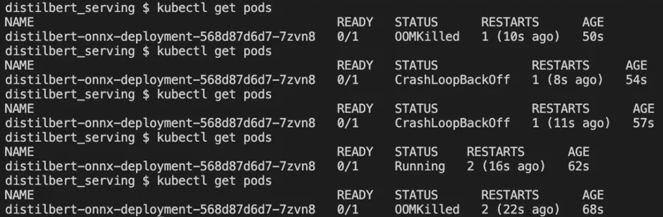
ONNX pod crashing with OOMKilled under 500Mi memory limit

To keep the comparison fair, I reran the PyTorch benchmark at 1Gi as well. The latency stayed essentially unchanged, confirming that the memory increase was not the driver of any performance difference.

The following results are from the PyTorch version.

PyTorch — short input, steady-state

PyTorch — medium input, steady-state

PyTorch — long input, steady-state

The following results are from the ONNX version.

ONNX — short input, steady-state

ONNX — medium input, steady-state

ONNX — long input, steady-state

Here is the results table.

Steady-state benchmark results (10 VUs, 120s, 1 pod)

The results indicate that ONNX is dramatically faster (the average latency dropped from 1.98 s to 598.72 ms) and provides much higher throughput (increased from 5.01 /s to 16.67 /s) compared to PyTorch. However, the performance gap becomes smaller as the input text gets longer, so when looking at the long test, the average latency only decreased 25% (3.07 s to 2.3 s) whereas it decreased nearly 70% (1.98 s to 598.72 ms) with the short test. Moreover, the throughput jumped 233% (5.01 /s to 16.67 /s) but with the long test, it only increased 34% (3.24 /s to 4.33 /s).

The total process time can be broken down into the fixed overhead and the actual inference, and the fixed overhead is where ONNX differs from PyTorch. With the short text, this advantage significantly affects the performance gap but as the text gets longer, the inference load starts dominating the process time which makes the gap small. ONNX reduces this fixed overhead through its static graph and operator fusion, which eliminates redundant computation that PyTorch performs dynamically on every request.

However, the dynamic graph PyTorch uses is necessary for model training and ONNX cannot be used to train models. So this experiment does not mean to prove that ONNX is absolutely better but instead they serve different purposes.

Cold-Start Benchmark Results

I additionally conducted cold-start tests to see how fast the pods can come up and become available. Being performant at inference is crucial but as seen in the previous blog, HPA cannot react fast enough to absorb the initial traffic spikes so being available fast is equally important to smoothly operate clusters and serve responsive applications.

I ran the following command to restart the deployment and timed how fast the pods become ready. It restarts the deployment and kubectl rollout status finishes when the pod becomes ready again so by timing this, I could measure how fast the pods get ready.

kubectl rollout restart deployment/distilbert-pytorch-deployment && \
time kubectl rollout status deployment/distilbert-pytorch-deployment

As soon as the pods became available, I ran the simple curl as follows and displayed the response time.

curl -w "\ntime_total: %{time_total}s\n" \
 -X POST "http://<LOAD_BALANCER_URL>:8080/analyze" \
 -H "Content-Type: application/json" \
 -d '{"text": "I love this movie!"}' \
 -o /dev/null -s

I ran the commands above three times each for PyTorch and ONNX for accurate testing.

The following results are from the PyTorch version.

1st Test:

PyTorch cold-start — run 1

PyTorch cold-start — run 1

2nd Test:

PyTorch cold-start — run 2

PyTorch cold-start — run 2

3rd Test

PyTorch cold-start — run 3

PyTorch cold-start — run 3

The following results are from the ONNX version.

1st Test:

ONNX cold-start — run 1

ONNX cold-start — run 1

2nd Test:

ONNX cold-start — run 2

ONNX cold-start — run 2

3rd Test:

ONNX cold-start — run 3

ONNX cold-start — run 3

The results are organized in the following table.

Cold-start results — average of 3 runs

Looking at the results table, the startup-to-readiness time didn’t differ significantly between PyTorch and ONNX. However, the first request latency drops nearly 95% from 1.88 seconds to 0.10 seconds and this significantly helps pods absorb the initial spikes. This connects directly to the finding from the previous blog: when HPA scales out new pods to absorb a traffic spike, those pods need to serve requests immediately after becoming ready. With PyTorch, that first request costs nearly 2 seconds. With ONNX, it costs 0.1 seconds.

Key Findings

Through this experiment, I found that the performance gap between PyTorch and ONNX is most significant when the input is short and the gap gradually gets smaller as the input gets longer. When the gap was most significant, the average latency dropped 70% and the throughput increased 232%. When it was least significant, the average latency dropped 25% and the throughput increased 33%. In the cold-start test, the first request latency decreased 95% while the startup-to-readiness time barely improved.

This observation suggests that ONNX provides clear performance advantages, but the magnitude depends on the workload. The drawbacks are that ONNX cannot be used for model training and it requires more memory and the docker image gets larger compared to the PyTorch version. Thus, this confirms that PyTorch and ONNX are used for different purposes and ONNX alone cannot solve all problems. Careful consideration is needed before adopting ONNX in production.

Conclusion

In this experiment, I benchmarked inference performance across three input sizes, comparing PyTorch against ONNX Runtime, an open-source inference engine. I found that the input length matters for the performance and understood why it behaves this way: ONNX compresses the overhead but as the input gets large, the actual inference starts dominating the process time.

The most notable finding from this experiment is that ONNX excels at handling the first request after a pod becomes ready, but does not meaningfully reduce the time it takes for a pod to start up. So ONNX is not a replacement for warm capacity. What it changes is that each newly ready pod becomes effective much faster. My current assumption is that regardless of the inference engine, keeping some pods idle during low-traffic periods is necessary. ONNX can then handle the initial spike more efficiently while HPA scales up the cluster.

Next, I plan to implement a CI/CD pipeline with GitHub Actions to automate image builds and deployments to EKS, removing manual steps and making the release process reproducible.