GCP-PDE — 30 Practice Questions to Crack Section 4 — Preparing and using data for analysis

Visualisation. ML. Sharing. No repeats. No mercy.

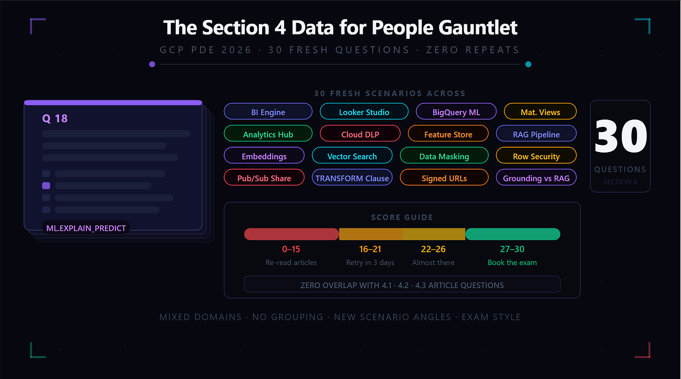
Section 4 is where data engineering meets the business. The warehouse is built. The lake is governed. Now the question is: can you get the data to the people who need it — fast enough for dashboards, smart enough for ML, safe enough for partners?

Every question below is a fresh scenario. None appear in the 4.1, 4.2, or 4.3 articles. Same tools, new angles, real exam pressure.

Q1 — Looker Studio: Extract Mode Trade-off

Cymbal’s operations team refreshes a Looker Studio dashboard 200 times per day. The underlying BigQuery query joins three tables and scans 800 GB each time. The data changes every 4 hours. The team switches to extract mode with a 4-hour refresh schedule. What is the trade-off they accept?

• A. Queries become slower — extract mode adds processing overhead
• B. Data in the dashboard may be up to 4 hours old — users viewing between refreshes see a snapshot, not live data
• C. The dashboard stops working for BigQuery datasets larger than 100 GB
• D. Extract mode costs more than direct query mode

Answer: B

• Extract mode caches the data at refresh time — between refreshes, users see the cached snapshot. If data changes 10 minutes after an extract, users won’t see it for up to 4 hours. This is the explicit trade-off: lower BigQuery cost vs data freshness. The 200 daily refreshes become 6 BigQuery queries per day (one every 4 hours) instead of 200. Extracts are faster to serve (A is wrong). BigQuery datasets over 100 GB are supported — the 100 MB limit is on the extract cache size, not the source (C is wrong). Extract mode reduces cost, not increases it (D is wrong).

Q2 — Cyclic Encoding

Cymbal’s demand forecasting model uses hour_of_day (0–23) as a feature. A data scientist encodes it as a raw integer: hour 23 = 23, hour 0 = 0. The model performs poorly because it treats 11 PM (23) as very different from midnight (0) even though they're adjacent. What is the correct fix?

• A. Normalise hour_of_day to 0–1 using min-max scaling
• B. One-hot encode hour_of_day — create 24 binary columns
• C. Apply cyclic encoding: sin(2π × hour / 24) and cos(2π × hour / 24) — two features that preserve the circular nature of time
• D. Remove hour_of_day — it adds noise to the model

Answer: C

• Hours form a cycle — hour 23 is adjacent to hour 0. A raw integer encoding treats the distance from 23 to 0 as 23 units, but the true distance is 1 unit. Cyclic encoding maps hours onto a circle using sin and cos — hour 23 and hour 0 are correctly represented as close together. Normalisation (A) still treats 23 and 0 as far apart. One-hot (B) creates 24 columns and loses the ordinal relationship entirely. Removing the feature (D) loses valuable temporal information — hour of day is highly predictive for retail demand.

Q3 — Materialised View: Smart Rewrite

Cymbal’s analyst runs this query: SELECT store_region, SUM(order_total) FROM order_facts WHERE order_date >= '2025-01-01' GROUP BY store_region. Unknown to the analyst, a materialised view exists: mv_regional_revenue which precomputes exactly SUM(order_total) GROUP BY store_region, order_date. The analyst's query references order_facts directly. What happens?

• A. The query scans the full order_facts table — the analyst must explicitly reference the materialised view
• B. BigQuery’s smart query rewrite automatically redirects the query to read from mv_regional_revenue — the analyst gets the fast precomputed result without knowing the view exists
• C. An error is returned — queries must reference the materialised view explicitly
• D. BigQuery runs both the full scan and the materialised view scan and returns whichever finishes first

Answer: B

• BigQuery’s smart query rewrite automatically redirects matching queries to materialised views — the analyst’s query pattern (SUM of order_total grouped by region with a date filter) matches the materialised view’s precomputed aggregation. The analyst never needs to know the view exists. This is one of the most powerful features of BigQuery materialised views — transparent acceleration. Full scan (A) would be the behaviour without materialised views. Explicit reference requirement © is wrong — that’s the whole point of smart rewrite. Running both (D) doesn’t exist as a BigQuery behaviour.

Q4 — Training-Serving Skew

Cymbal’s churn model was trained with order_total normalised using the training dataset's min ($0.01) and max ($49,999). Six months later, a major corporate customer places orders worth $250,000. At serving time, the model receives order_total = 250000. Without the TRANSFORM clause, what is the normalised value and why is it a problem?

• A. The value is normalised to 1.0 — the maximum is capped, no problem
• B. The value normalises to approximately 5.0 — outside the 0–1 range the model was trained on, causing unexpected prediction behaviour
• C. BigQuery automatically clips the value to the training range — no action needed
• D. The serving pipeline recomputes min/max from live data — always correctly normalised

Answer: B

• Min-max normalisation: (250000 - 0.01) / (49999 - 0.01) ≈ 5.0. The model was trained on values in [0, 1] — receiving a value of 5.0 puts the input outside the distribution the model learned. Predictions become unreliable. This is training-serving skew. The fix: use the TRANSFORM clause in BigQuery ML — it stores the training-time min/max and applies the same normalisation at serving time, regardless of new data ranges. BigQuery doesn't auto-clip values (C). The serving pipeline should NOT refit the scaler (D) — that's exactly the skew problem.

Q5 — Analytics Hub: Subscriber Billing

Cymbal publishes a 2 TB customer analytics dataset to Analytics Hub. The marketing team at Cymbal subscribes (internal exchange) and runs 100 queries per day, each scanning the full 2 TB linked dataset. Cymbal’s analytics team (another internal team) also subscribes and runs 50 queries per day. How are the query costs distributed?

• A. All query costs are billed to Cymbal’s publishing project since they own the source data
• B. Marketing team pays for their 100 queries (billed to their project); analytics team pays for their 50 queries (billed to their project); Cymbal’s publishing project pays only storage
• C. Costs are split equally between all three projects
• D. Analytics Hub queries are free — no billing applies

Answer: B

• Analytics Hub uses the requester-pays model. Each subscriber’s queries are billed to their own project. The marketing team’s project pays for 100 queries × 2 TB = 200 TB scanned. The analytics team’s project pays for 50 queries × 2 TB = 100 TB scanned. Cymbal’s publishing project pays only for the 2 TB storage. This is one of Analytics Hub’s primary commercial advantages — the publisher’s bill doesn’t scale with subscriber usage.

Q6 — BI Engine: Preferred Tables

Cymbal has a 20 GB BI Engine reservation for their analytics project. The project has three dashboards: Executive (queries 3 GB of data), Operations (queries 8 GB), and Regional (queries 15 GB). All three need sub-second response. The 20 GB reservation is insufficient to cache all three simultaneously. Which configuration prioritises the most business-critical dashboard?

• A. BI Engine caches automatically — no configuration needed
• B. Configure preferred tables for the Executive dashboard’s underlying tables — BI Engine prioritises caching them; Operations and Regional fall back to standard BigQuery for the portion that doesn’t fit
• C. Increase the BI Engine reservation to 26 GB to fit all three dashboards
• D. Create separate BI Engine reservations for each dashboard

Answer: B

• BI Engine preferred tables let you specify which BigQuery tables are prioritised for caching. The Executive dashboard (3 GB) is fully cached with priority. The remaining 17 GB accommodates most of Operations (8 GB). Regional (15 GB) partially caches. If the 3 GB Executive tables are designated as preferred, they’re always in memory — sub-second for the CFO’s board meeting. Auto-caching (A) doesn’t prioritise business criticality — BI Engine caches based on access frequency. Increasing to 26 GB © works but costs more — the question asks for the configuration approach. Separate reservations per dashboard (D) is not a supported BI Engine configuration.

Q7 — k-means Clustering in BigQuery ML

Cymbal’s marketing team wants to segment customers into behavioural groups for targeted campaigns. They have 5 million customers with features: avg_order_value, purchase_frequency, preferred_category, days_since_last_purchase. No predefined labels exist. Which BigQuery ML model type is correct?

• A. LOGISTIC_REG — classify each customer into a predefined segment
• B. ARIMA_PLUS — forecast which segment each customer will move to
• C. KMEANS — unsupervised clustering groups customers by feature similarity without predefined labels
• D. DNN_CLASSIFIER — deep neural network for complex customer pattern recognition

Answer: C

• No predefined labels = unsupervised learning = k-means clustering. K-means groups customers with similar feature values into clusters — the model discovers the segments rather than being told what they are. Logistic regression (A) requires predefined binary/multi-class labels — there are none. ARIMA_PLUS (B) is time-series forecasting — not customer segmentation. DNN Classifier (D) requires labelled training data — “which segment does this customer belong to?” — but the segments don’t exist yet.

**Q8 — Query Performance: SELECT ***

Cymbal’s Looker Studio dashboard runs SELECT * FROM order_facts WHERE order_date = '2025-06-01'. The order_facts table has 200 columns and is 50 TB. The query scans 50 GB per run (one day's partition) but takes 45 seconds. Investigation reveals the dashboard only uses 8 of the 200 columns. What is the most impactful fix?

• A. Add more clustering columns to order_facts
• B. Enable BI Engine — it accelerates SELECT * queries
• C. Replace SELECT * with SELECT col1, col2, col3, col4, col5, col6, col7, col8 — BigQuery is columnar; selecting only 8 of 200 columns reduces bytes scanned from 50 GB to approximately 2 GB
• D. Partition the table more finely — hourly instead of daily

Answer: C

• BigQuery is a columnar storage engine — it reads only the columns referenced in the query. SELECT * reads all 200 columns even if the application uses only 8. Selecting only the 8 needed columns reduces bytes scanned by approximately 96% (200 → 8 columns). This is the single most impactful change for wide-table queries. Additional clustering (A) helps with row filtering, not column pruning. BI Engine (B) caches results but doesn't fix the root cause of unnecessary column scanning. Hourly partitioning (D) helps time-filtered queries but doesn't address the column problem.

Q9 — Cloud DLP: Discovery vs De-identification

Cymbal ingests a new supplier dataset into BigQuery. The data engineering team suspects it contains PII but doesn’t know exactly which columns. They need to: (1) identify which columns contain PII, (2) mask the PII before the dataset is shared with the analytics team. Which Cloud DLP operations address each step?

• A. (1) DLP tokenisation scan, (2) DLP redaction
• B. (1) DLP inspection/discovery scan — identifies PII column patterns, (2) DLP de-identification transformation — masks or transforms the detected PII values
• C. (1) Policy Tags — automatically detect PII, (2) DLP masking rule
• D. (1) Dataplex quality scan, (2) DLP tokenisation

Answer: B

• Cloud DLP has two distinct modes: inspection (discovery) scans a dataset to identify which fields contain PII patterns (credit cards, emails, national IDs, etc.) — step 1. De-identification applies transformation rules (redaction, tokenisation, generalisation) to mask the detected values — step 2. Policy Tags © enforce access control but don’t detect PII automatically — they must be applied after discovery. Dataplex quality scans (D) check data rules (nulls, ranges) — not PII detection. Tokenisation is a de-identification method, not a scan type (A is wrong order).

Q10 — RAG: Chunking Strategy

Cymbal’s RAG system indexes 500 policy documents for the AI customer support assistant. Each document is 20–50 pages. The team is debating chunk sizes: 100 tokens vs 500 tokens vs 2,000 tokens. Which consideration is most important for chunk size selection?

• A. Larger chunks are always better — more context per retrieval
• B. Smaller chunks are always better — more precise retrieval
• C. Chunk size must balance retrieval precision (smaller chunks = more specific matches) and context completeness (larger chunks = more context for the LLM to answer from) — 500 tokens is a common practical balance; domain and document structure should guide the choice
• D. Chunk size doesn’t matter — the LLM reads the entire document regardless

Answer: C

• Chunk size is a genuine engineering trade-off. Very small chunks (100 tokens) retrieve precisely but may not contain enough context for the LLM to generate a complete answer. Very large chunks (2,000 tokens) contain more context but may match irrelevant sections alongside relevant ones — diluting retrieval precision. 500 tokens is a commonly recommended starting point, with tuning based on the specific document structure and query patterns. “Larger is always better” (A) and “smaller is always better” (B) are both wrong — it depends on the use case. The LLM does not read entire documents in RAG — only the retrieved chunks are included in the prompt (D is wrong).

Q11 — Policy Tags on Linked Datasets

Cymbal’s source BigQuery dataset has Policy Tags applied to customer_email (PII tag) and national_id (sensitive tag). The marketing team subscribes to this dataset via Analytics Hub and gets a linked dataset in their project. The marketing team's analysts do not have Fine-Grained Reader on the PII or sensitive tags. What do the analysts see when they query customer_email and national_id from the linked dataset?

• A. The raw values — Policy Tags only apply to the source dataset, not linked datasets
• B. NULL for both columns — Policy Tags applied to the source dataset automatically enforce on linked datasets
• C. An error message — linked datasets cannot contain Policy Tag-restricted columns
• D. The columns are hidden from the schema — they don’t appear in the linked dataset at all

Answer: B

• Policy Tags from the source dataset are inherited by linked datasets in Analytics Hub. Subscribers without Fine-Grained Reader on the relevant tags see NULL for those columns — exactly as they would if querying the source dataset directly without the role. This is one of Analytics Hub’s governance strengths — the publisher’s security model extends automatically to all subscribers. The columns remain visible in the schema (D is wrong) and don’t cause errors (C is wrong), and tags absolutely apply to linked datasets (A is wrong).

Q12 — Feature Store: When to Use

Cymbal’s recommendation engine serves product suggestions to users as they browse the app. The model needs 15 precomputed features per user including avg_session_duration, top_3_categories, and purchase_probability_score. These features are computed daily in BigQuery. The serving latency requirement is under 50ms. BigQuery query latency for these features is 800ms. Which solution bridges this gap?

• A. Cache features in BigQuery BI Engine — sub-second response
• B. Precompute features daily in BigQuery and serve from Vertex AI Feature Store — sub-50ms online serving via the Feature Store API
• C. Run BigQuery ML inference inline at serving time — ML.PREDICT returns results in under 50ms
• D. Use Memorystore Redis with a 24-hour TTL — cache features per user_id

Answer: B

• Vertex AI Feature Store is the purpose-built solution for serving precomputed ML features with low latency at serving time. Features computed in BigQuery are written to Feature Store; the online serving API retrieves them in under 20ms. BI Engine (A) caches query results for BI dashboards — not for ML feature serving APIs. ML.PREDICT inline (C) still runs BigQuery queries at 800ms — that's the problem being solved. Memorystore (D) works technically but lacks feature versioning, lineage tracking, and point-in-time correctness guarantees that Feature Store provides. For production ML serving, Feature Store is the correct answer.

Q13 — Dry Run for Cost Validation

Cymbal’s data engineering team is deploying a new dashboard query against a 500 TB table. They want to verify that partitioning is working correctly and the query won’t scan the full table before running it in production. Which BigQuery feature provides this validation without incurring query costs?

• A. Run the query against a 1% sample using TABLESAMPLE
• B. Check the execution plan in the BigQuery console after running the query
• C. Submit the query with the --dry_run flag — BigQuery returns the estimated bytes to be processed without executing the query
• D. Run EXPLAIN before the query to see the execution plan

Answer: C

• A BigQuery dry run estimates the bytes that would be processed without actually running the query or incurring costs. If partition pruning is working, a daily-partitioned table with a date filter should show only the filtered partition’s size — not 500 TB. TABLESAMPLE (A) runs an actual query (incurs cost) on a random subset — doesn’t validate partitioning. Checking the execution plan (B) requires running the query first — incurs the full cost. BigQuery doesn’t support an EXPLAIN command (D) — the execution plan is available post-run only.

Q14 — Signed URLs: Appropriate Use Case

Cymbal’s legal team needs to share a specific BigQuery export (a 2 GB CSV file of anonymised research data) with an academic partner. The academic partner has no GCP account. Access should expire after 48 hours. Which mechanism is correct?

• A. Create an Analytics Hub listing — the academic partner subscribes
• B. Grant the academic partner roles/storage.objectViewer on the Cloud Storage bucket
• C. Generate a signed URL for the specific Cloud Storage object with a 48-hour expiry — share the URL with the partner
• D. Export to a public Cloud Storage bucket accessible to anyone with the link

Answer: C

• Signed URLs embed authentication in the URL itself — no GCP account required. The 48-hour expiry means access automatically terminates. Analytics Hub (A) requires a GCP organisation — the academic partner has none. IAM roles (B) require the partner to have a Google identity and a GCP project. A public bucket (D) has no access control or expiry — anyone who finds the URL can access it indefinitely, which is a security risk.

Q15 — INFORMATION_SCHEMA for Cost Analysis

Cymbal’s BigQuery costs spike by 300% in one week. The data team needs to identify which queries and which users are responsible. Which BigQuery feature provides this information?

• A. Cloud Monitoring — check BigQuery slot utilisation dashboards
• B. Query INFORMATION_SCHEMA.JOBS_BY_PROJECT — filter by the week in question, order by total_bytes_billed DESC — identify the most expensive queries, their authors, and their query text
• C. Check the BigQuery execution plan for each table
• D. Review Cloud Audit Logs for BigQuery job events

Answer: B

• INFORMATION_SCHEMA.JOBS_BY_PROJECT contains metadata for every BigQuery job: total_bytes_billed, user_email, query, start_time, job_id. A simple ORDER BY total_bytes_billed DESC LIMIT 20 on the previous week's jobs immediately identifies the culprits. Cloud Monitoring (A) shows slot utilisation at the infrastructure level — not individual query attribution. Execution plans (C) are per-query, post-run details — not a cost analysis tool. Cloud Audit Logs (D) contains job events but is harder to query for cost analysis than INFORMATION_SCHEMA.

Q16 — One-Hot Encoding Limitation

Cymbal’s product recommendation model uses product_id as a feature. The product catalogue has 80,000 distinct products. A junior data scientist proposes one-hot encoding: create 80,000 binary columns. Why is this problematic and what is the correct alternative?

• A. One-hot encoding is fine for any cardinality — proceed as suggested
• B. 80,000 binary columns creates an extremely high-dimensional sparse vector — most values are 0 for any given row; memory-intensive and informationally inefficient; use a learned embedding that represents each product as a dense low-dimensional vector (e.g., 64 dimensions)
• C. Use label encoding instead — assign each product_id an integer from 1 to 80,000
• D. Remove product_id from features entirely — it's too high cardinality to be useful

Answer: B

• One-hot encoding 80,000 products creates an 80,000-dimensional vector where 79,999 values are 0 for any given product — extremely sparse. Training on this representation is computationally expensive and doesn’t capture product similarity. Learned embeddings represent each product as a dense 64-dimensional vector — similar products end up with similar embeddings. Label encoding © assigns arbitrary integers implying false ordinal relationships (product #1 is not “less than” product #2). Removing the feature entirely (D) loses valuable product identity information.

Q17 — Cross-Project Pub/Sub Sharing

Cymbal’s warehouse management system (in cymbal-wms project) publishes restock events to a Pub/Sub topic. The logistics partner's system (in partner-logistics GCP project) needs to consume these events in real-time. Which configuration enables this?

• A. Export Pub/Sub messages to Cloud Storage and share a signed URL with the partner
• B. Create a Pub/Sub subscription in partner-logistics project on Cymbal's topic — grant the partner's service account roles/pubsub.subscriber on the subscription
• C. Use Analytics Hub to publish the Pub/Sub topic as a listing
• D. Use Datastream to replicate Pub/Sub messages to the partner’s project

Answer: B

• Pub/Sub supports cross-project subscriptions. The partner creates a subscription on Cymbal’s topic in their own project, and Cymbal grants their service account the roles/pubsub.subscriber role on that subscription. Messages are delivered to the partner's subscriber in real-time. Signed URL exports (A) are for Cloud Storage files — not real-time event streams. Analytics Hub (C) is for BigQuery datasets, not Pub/Sub topics. Datastream (D) is for database CDC replication — not Pub/Sub message routing.

Q18 — ML.EXPLAIN_PREDICT Use Case

Cymbal’s fraud detection model flags order #12345 as high risk (fraud score: 0.94). The fraud operations team needs to understand why this specific order received a high score — which features drove the prediction — before deciding whether to block the transaction. Which BigQuery ML function provides this?

• A. ML.EVALUATE — returns model-level performance metrics
• B. ML.PREDICT with EXPLAIN option — returns predictions with feature contributions
• C. ML.EXPLAIN_PREDICT — returns Shapley value-based feature importance for each individual prediction, showing which features contributed most to the fraud score
• D. ML.FEATURE_INFO — returns feature statistics from the training data

Answer: C

• ML.EXPLAIN_PREDICT runs inference and returns Shapley values for each feature on each prediction — it shows that for order #12345, the high fraud score was driven by unusual_shipping_address (contribution: +0.42), first_time_buyer (+0.28), and order_placed_at_3am (+0.19). ML.EVALUATE (A) gives model-wide metrics like AUC — not per-prediction explanations. ML.PREDICT alone (B) returns the score but not the feature contributions. ML.FEATURE_INFO (D) is not a standard BigQuery ML function.

Q19 — Require Partition Filter

Cymbal’s clickstream_events table is 200 TB and date-partitioned. Analysts occasionally forget to include a date filter and accidentally run full-table scans — costing thousands of dollars. What BigQuery configuration prevents this?

• A. Apply column-level Policy Tags to the partition column — analysts without access can’t query it
• B. Set require_partition_filter = TRUE on the table — BigQuery rejects any query that doesn't include a filter on the partition column
• C. Create a row-level security policy that returns no rows unless a date filter is present
• D. Set a BigQuery project-level cost control that caps bytes billed per query at 1 TB

Answer: B

• require_partition_filter = TRUE is a table-level option that forces every query to include an explicit filter on the partition column. Queries without the filter are rejected with an error before scanning any data — zero cost, clear error message. Policy Tags (A) restrict who can access a column — not whether a filter is required. Row-level security (C) can't enforce filter presence — it filters rows, not query structure. Cost caps (D) fail the query after it's already scanned the data — reactive, not preventive.

Q20 — ARIMA_PLUS: Holiday Detection

Cymbal uses BigQuery ML’s ARIMA_PLUS model to forecast daily order volume per store. The model performs well for normal weeks but consistently underestimates orders during UK public holidays. Which ARIMA_PLUS option addresses this?

• A. Add is_holiday as a manual feature in the training query
• B. Set holiday_region = 'GB' in the model OPTIONS — ARIMA_PLUS automatically incorporates UK public holiday effects into the seasonality decomposition
• C. Retrain the model with only holiday-period data
• D. Use BOOSTED_TREE_REGRESSOR instead — it handles holiday effects better

Answer: B

• ARIMA_PLUS has built-in holiday effect modelling. Setting holiday_region = 'GB' (or other supported country codes) automatically incorporates public holiday patterns into the time-series decomposition — no manual feature engineering required. Adding is_holiday manually (A) works but requires maintaining a holiday calendar and re-engineering the feature — unnecessary when ARIMA_PLUS handles this natively. Retraining on only holiday data (C) would overfit to holidays and perform poorly on normal days. Boosted trees (D) would require extensive manual temporal feature engineering to match ARIMA_PLUS's built-in seasonal handling.

Q21 — Vector Search: Cosine vs Euclidean

Cymbal’s product search uses text embeddings. A customer searches “lightweight running shoes for marathon training.” The system retrieves the top-10 most similar products from 100,000 embeddings. Which distance metric is most appropriate for comparing text embeddings?

• A. Euclidean distance — measures absolute distance in vector space
• B. Cosine similarity — measures the angle between vectors; direction (meaning) matters more than magnitude (length) for text
• C. Manhattan distance — sum of absolute differences per dimension
• D. Dot product — measures the raw alignment between vectors

Answer: B

• Text embeddings encode semantic meaning in the direction of the vector, not its magnitude. Two descriptions of the same concept produce vectors pointing in similar directions — even if their magnitudes differ (longer descriptions may produce larger magnitude vectors). Cosine similarity captures directional alignment regardless of magnitude — ideal for text similarity. Euclidean distance (A) treats magnitude differences as meaningful — a longer description would appear less similar even if semantically identical. Manhattan © is rarely used for high-dimensional embeddings. Dot product (D) is affected by magnitude — biases toward longer texts.

Q22 — Analytics Hub: Authorised View as Listing Source

Cymbal wants to publish inventory data to franchise partners via Analytics Hub. The source inventory_facts table contains sensitive supplier cost prices (supplier_cost) that partners must never see. All other columns can be shared. What is the correct listing source?

• A. Publish inventory_facts directly and apply Policy Tags to supplier_cost — partners see NULL for that column
• B. Create an authorised view on inventory_facts that excludes supplier_cost — publish the authorised view as the Analytics Hub listing source
• C. Use Cloud DLP to redact supplier_cost in real-time as partners query it
• D. Create a separate BigQuery table without supplier_cost and publish it

Answer: B

• An authorised view selects all columns except supplier_cost from inventory_facts. The view is published as the listing source — partners subscribe to the view and never have access to the underlying table or the excluded column. Policy Tags (A) return NULL for the column — partners know the column exists and that they're being restricted. The authorised view approach (B) completely hides the column from the schema — cleaner and more secure. DLP real-time redaction (C) adds latency and complexity for something an authorised view handles structurally. A separate table (D) creates a data copy that must be kept in sync — operational overhead.

Q23 — Normalisation: When Not To

Cymbal’s fraud model includes a binary feature is_first_time_buyer (0 or 1). A data scientist applies z-score standardisation to all features uniformly, including this binary column. What is the problem?

• A. Z-score standardisation doesn’t work on binary values — it throws an error
• B. Standardising a binary column transforms it from {0, 1} to approximately {-0.5, +1.5} — the model still works but the transformed values have no natural interpretation; for tree-based models (like XGBoost), this transformation is unnecessary and adds no value
• C. The binary column becomes continuous after standardisation — the model cannot handle it
• D. Standardisation of binary columns causes data leakage

Answer: B

• Z-score standardisation of a binary column technically works without errors, but for tree-based models (XGBoost, random forests), which split on feature values, transforming {0, 1} to {-0.5, +1.5} doesn’t change the relative ordering — the model splits identically. The transformation is unnecessary overhead. For linear models (logistic regression), standardising all features including binary ones is common practice for convergence stability. The key point: normalisation decisions should be model-type-aware, not applied uniformly. No error is thrown (A is wrong). The column remains a valid input (C is wrong). No data leakage (D is wrong).

Q24 — Analytics Hub: Discovery Without Access

Cymbal’s data governance team wants all employees to be able to browse the internal Analytics Hub exchange and see what data products are available — their descriptions, schemas, freshness SLAs, and owners — without being able to subscribe or query any data. Which role achieves this?

• A. roles/analyticshub.subscriber — allows browsing and subscribing
• B. roles/analyticshub.viewer — allows browsing listings without subscribing or accessing data
• C. roles/bigquery.metadataViewer — allows seeing BigQuery metadata across projects
• D. roles/dataplex.dataReader — allows reading data lake assets

Answer: B

• roles/analyticshub.viewer is specifically designed for discovery without access — employees can see all listings, read descriptions, view schemas, and check freshness commitments, but cannot subscribe or query any data. Subscriber role (A) adds subscription rights — not appropriate for read-only browsing. BigQuery metadata viewer (C) shows BigQuery table metadata within a project — not Analytics Hub listing metadata. Dataplex data reader (D) grants access to data lake assets — unrelated to Analytics Hub listing discovery.

Q25 — BigQuery ML: Batch vs Online Prediction

Cymbal’s churn model must serve two use cases: (1) overnight batch scoring of all 5 million customers to prioritise the next day’s retention campaign (results in BigQuery by 6 AM), (2) real-time scoring of a customer the moment they contact customer support (result within 200ms). Which prediction approach is correct for each use case?

• A. ML.PREDICT in BigQuery for both — BigQuery handles batch and real-time
• B. ML.PREDICT in BigQuery for use case 1 (batch overnight scoring); Vertex AI online prediction endpoint for use case 2 (real-time under 200ms)
• C. Vertex AI batch prediction for use case 1; ML.PREDICT for use case 2
• D. Vertex AI online prediction endpoint for both

Answer: B

• BigQuery ML.PREDICT on 5 million rows overnight is exactly the right tool — it's a batch SQL operation, runs efficiently at scale, and results are in BigQuery by 6 AM for the campaign team. For real-time 200ms serving, BigQuery query latency (seconds) is incompatible — the model must be deployed to a Vertex AI online prediction endpoint that responds in milliseconds. Vertex AI batch prediction (C) for use case 1 would require exporting data from BigQuery — unnecessary when ML.PREDICT runs in-place. Vertex AI online endpoints (D) for 5 million rows nightly is cost-inefficient compared to BigQuery ML.PREDICT.

Q26 — Looker PDTs vs BigQuery Materialised Views

Cymbal uses Looker for enterprise BI. The data team is deciding whether to use Looker Persistent Derived Tables (PDTs) or BigQuery materialised views for precomputing a complex revenue cohort analysis. Which consideration determines the correct choice?

• A. PDTs are always faster than materialised views
• B. If the transformation logic is owned and maintained by the Looker/BI team in LookML, use PDTs. If the transformation is owned by the data engineering team in SQL and serves multiple tools beyond Looker, use BigQuery materialised views
• C. BigQuery materialised views are free; PDTs incur additional Looker licensing costs
• D. PDTs support incremental refresh; BigQuery materialised views do not

Answer: B

• The ownership and consumption model determines the correct choice. PDTs are Looker-native — defined in LookML, managed in Looker, visible only within Looker. If the BI team owns the logic and it’s Looker-specific, PDTs are the right tool. BigQuery materialised views are warehouse-native — defined in SQL, managed in BigQuery, accessible from any tool (Looker Studio, Tableau, Connected Sheets, Python). If the engineering team owns the logic and multiple tools need it, materialised views are correct. Speed (A) depends on the query — no universal rule. Licensing costs © aren’t the driver for this decision. BigQuery materialised views do support incremental refresh for supported query patterns (D is wrong).

Q27 — Grounding vs RAG

Cymbal’s AI assistant needs to answer questions about product availability using Cymbal’s real-time inventory data. The inventory data is in BigQuery, updated every 15 minutes. The team is choosing between RAG with a BigQuery-backed knowledge base vs Vertex AI Grounding with Cymbal’s own data source. What is the key architectural difference?

• A. RAG uses open-source models; Vertex AI Grounding uses Gemini only
• B. RAG retrieves from a pre-indexed static vector store — best for document corpora that change infrequently. Vertex AI Grounding can connect to live data sources — better for frequently updated structured data like inventory
• C. RAG is more accurate than Vertex AI Grounding for all use cases
• D. There is no difference — both architectures produce identical results

Answer: B

• The key distinction is data freshness and structure. RAG retrieves from an indexed vector store — if inventory data changes every 15 minutes, the index must be rebuilt every 15 minutes (operationally complex). Vertex AI Grounding can connect to BigQuery or other live data sources directly — the AI queries real-time data as part of the grounding process. For policy documents that change monthly, RAG with a vector store is excellent. For live operational data updated every 15 minutes, Vertex AI Grounding with a BigQuery connection is more appropriate. Both use Gemini (A is wrong). Neither is universally more accurate ©. They are architecturally distinct (D is wrong).

Q28 — Row-Level Security vs Authorised View

Cymbal has one sales_facts table shared by 50 regional managers (each sees their own region) and 5 executives (who see all regions). The most maintainable solution at scale (new managers, new regions added quarterly) is required. Which mechanism is correct?

• A. Create 50 authorised views — one per region — grant each manager access to their view
• B. Row access policies on sales_facts — a single policy maps each user to their region via IAM group membership; executives are in an "all regions" group; new managers/regions require only IAM group updates, not schema or view changes
• C. Partition sales_facts by region and grant partition-level IAM per manager
• D. Export each region’s data to a separate BigQuery dataset per manager

Answer: B

• Row access policies scale elegantly — one policy definition, IAM group membership drives the data filtering. Adding a new manager means adding them to the regional IAM group. Adding a new region means adding it to the policy filter. No views to create, no schemas to change. 50 authorised views (A) require maintenance for every schema change across all 50 views — poor scalability. Partition-level IAM © is not a supported BigQuery primitive. Separate datasets per manager (D) create data duplication and synchronisation overhead — 50 copies of regional data.

Q29 — Data Masking: SHA-256 Hash Use Case

Cymbal needs to share customer transaction data with a fraud research team. The team needs to be able to: link transactions from the same customer across different tables (join on customer identity), but must not be able to identify who the actual customer is. Which Cloud DLP masking technique satisfies both requirements?

• A. Nullification — replace customer_id with NULL in both tables
• B. Redaction — replace customer_id with [REDACTED] in both tables
• C. SHA-256 deterministic hash — the same customer_id always produces the same hash in both tables; the research team can join on the hash without knowing the real identity
• D. Date year-only masking — replace customer_id with just the first 4 characters

Answer: C

• SHA-256 deterministic hashing produces the same output for the same input — customer_id = 'CUST-12345' always hashes to the same value. The research team can join transactions from different tables using the hashed ID without ever knowing the real identity. Nullification (A) makes all rows look identical (NULL = NULL in joins) — joining is impossible. Redaction (B) replaces all values with the same literal [REDACTED] — same problem as nullification for joins. Date year-only (D) is for DATE columns — not applicable to ID fields.

Q30 — Full Section 4 Scenario

Cymbal is building a unified AI retail intelligence system. Requirements: (1) the executive dashboard must load in under 1 second showing last 90 days of revenue; (2) a churn prediction model must score all customers weekly and serve real-time scores at checkout in under 100ms; (3) an AI assistant must answer customer support questions using Cymbal’s return policies (updated monthly); (4) the franchise partner network must query regional performance data from their own GCP projects. Which architecture satisfies all four requirements?

• A. BigQuery for everything — dashboards, ML, RAG, and partner sharing
• B. BI Engine + materialised views (req 1); BigQuery ML weekly batch + Vertex AI Feature Store online serving (req 2); RAG with ML.EMBED_TEXT + VECTOR_SEARCH + ML.GENERATE_TEXT (req 3); Analytics Hub linked datasets (req 4)
• C. Looker Studio direct query (req 1); Dataflow ML pipeline (req 2); fine-tuned Gemini (req 3); CSV exports to partners (req 4)
• D. BI Engine (req 1); Vertex AI AutoML (req 2); Vertex AI Search (req 3); shared BigQuery IAM viewer (req 4)

Answer: B

• Working through each: (1) BI Engine caches the materialised view result in memory — sub-second dashboard. (2) BigQuery ML ML.PREDICT runs the weekly batch; Vertex AI Feature Store serves precomputed features at sub-100ms for real-time checkout scoring. (3) RAG: ML.EMBED_TEXT generates embeddings for policy documents, VECTOR_SEARCH retrieves relevant chunks, ML.GENERATE_TEXT generates grounded answers — when policies update monthly, just re-embed the new document. (4) Analytics Hub: partners subscribe in their own GCP projects, pay for their own queries, access is revocable. Option C uses direct query (fails req 1 latency), fine-tuning (fails req 3 — monthly updates would require monthly retraining), and CSV exports (fails req 4 — not live queryable data). Option D doesn't use Feature Store for req 2 (Vertex AI AutoML is a training tool, not a serving solution) and shared IAM viewer (fails req 4's billing separation).

How Did You Score?

• 27–30 — Section 4 mastered. You’re thinking in systems, not just tools.
• 22–26 — Strong. Review the questions you missed — the trap is usually in one specific constraint.
• 16–21 — The concepts are there. Revisit 4.1 (BI Engine + troubleshooting), 4.2 (TRANSFORM clause + RAG steps), and 4.3 (zero-copy + subscriber billing).
• Below 16 — Go back to Sections 4.1–4.3 before retrying.

The next practice set covers Section 5 — Maintaining and Automating.