【Reproduction】【macOS Tahoe 26.0.1】Bayer Sorter — Simulating Reference Design

MacBook Pro

[embed]Bayer sorter The bayer sorter challenge involves the design of a Si3N4 metasurface to split light in a wavelength-dependent way, so…invrs-io.github.io

1. Environment Setup 2. Execute the Complete Code Acknowledgments and References

1. Environment Setup

Create a clean Conda environment to run the Bayer Sorter simulation with all necessary dependencies.

name: invrs
channels:
  - conda-forge
  - defaults
dependencies:
  # Core Python
  - python=3.10
  - pip
  - numpy
  - scipy
  - pandas
  - matplotlib
  - tqdm
  - pytest
  - scikit-image
  - git

  # JAX (CPU version)
  - jax
  - jaxlib

  # Install remaining dependencies via pip
  - pip:
      - invrs-gym
      - invrs-opt
      - ceviche
      - optax
      - flax
      - totypes
      - rich
      - ccmaps

$ conda env create -f env.yml
$ conda activate invrs

$ git clone https://github.com/invrs-io/gym.git
$ git clone https://github.com/invrs-io/leaderboard.git

$ cd gym
$ pip install -e .
$ cd ../leaderboard
$ pip install -e .

↪Back to the content⤴

2. Execute the Complete Code

Run the full Bayer Sorter simulation to reproduce the results, including visualization of transmission and focal-plane fields.

2–1. Run the whole script below

"""
Bayer sorter visualization with demo_outputs saved to 'demo_outputs' folder.
"""

import os
import matplotlib.pyplot as plt
import numpy as onp
from skimage import measure
import dataclasses
import jax.numpy as jnp
from invrs_gym.challenges.bayer import challenge as bayer_challenge
import jax
import ccmaps
# -------------------------------
# Ensure output folder exists
# -------------------------------
os.makedirs("demo_outputs", exist_ok=True)
# -------------------------------
# Load and plot design
# -------------------------------
design = onp.genfromtxt("../../../gym/reference_designs/bayer/zou.csv", delimiter=",")
# design = onp.genfromtxt("./solutions/220607_zou_00.csv", delimiter=",")
plt.figure(figsize=(3, 3))
ax = plt.subplot(111)
im = plt.imshow(1 - design, cmap="gray")
im.set_clim([-2, 1])
ax.set_xticks([])
ax.set_yticks([])
for c in measure.find_contours(design):
    plt.plot(c[:, 1], c[:, 0], 'k', lw=1)
plt.savefig("demo_outputs/design_plot.png", dpi=300)
plt.close()
# -------------------------------
# Initialize challenge
# -------------------------------
challenge = bayer_challenge.bayer_sorter(
    sim_params=dataclasses.replace(
        bayer_challenge.BAYER_SIM_PARAMS,
        approximate_num_terms=800,
        wavelength=jnp.arange(0.405, 0.7, 0.02),
    )
)
params = challenge.component.init(jax.random.PRNGKey(0))
assert params["density_metasurface"].shape == design.shape
params["density_metasurface"].array = design
response, aux = jax.jit(challenge.component.response)(params)
# -------------------------------
# Transmission plots
# -------------------------------
transmission = onp.mean(response.transmission, axis=-2)
transmission_blue_pixel = transmission[:, 0]
transmission_green_pixel = transmission[:, 1] + transmission[:, 2]
transmission_red_pixel = transmission[:, 3]
plt.plot(response.wavelength, transmission_blue_pixel, "bo-", lw=3)
plt.plot(response.wavelength, transmission_green_pixel, "go-", lw=3)
plt.plot(response.wavelength, transmission_red_pixel, "ro-", lw=3)
plt.xlabel("Wavelength")
plt.ylabel("Sub-pixel transmission")
plt.ylim(-0.05, 0.7)
plt.savefig("demo_outputs/transmission_plot.png", dpi=300)
plt.close()
# -------------------------------
# Field intensity plots
# -------------------------------
x, y = aux["coordinates_xy"]
x = jnp.squeeze(x, axis=0)
y = jnp.squeeze(y, axis=0)
ex, ey, ez = aux["efield_xy"]
intensity = jnp.abs(ex)**2 + jnp.abs(ey)**2 + jnp.abs(ez)**2
intensity = jnp.mean(intensity, axis=-1)  # Average over polarizations
fig, axs = plt.subplots(ncols=5, nrows=3, figsize=(9, 7))
axs = axs.flatten()
for i, wavelength in enumerate(response.wavelength):
    cmap = ccmaps.cmap_for_wavelength(wavelength_nm=wavelength * 1000)
    axs[i].pcolormesh(x, y, intensity[i, :, :], cmap=cmap)
    axs[i].set_ylim(axs[i].get_ylim()[::-1])
    axs[i].axis("equal")
    axs[i].axis(False)
    axs[i].plot([jnp.amin(x), jnp.amax(x)], [jnp.mean(y), jnp.mean(y)], "w--", lw=1)
    axs[i].plot([jnp.mean(x), jnp.mean(x)], [jnp.amin(y), jnp.amax(y)], "w--", lw=1)
    axs[i].set_title(f"$\lambda$={wavelength:.3f}$\mu$m", fontsize=10)
plt.subplots_adjust(wspace=0.05, hspace=0.25)
plt.savefig("demo_outputs/intensity_maps.png", dpi=300)
plt.close()

$ cd challenges/bayer_sorter/
$ python demo.py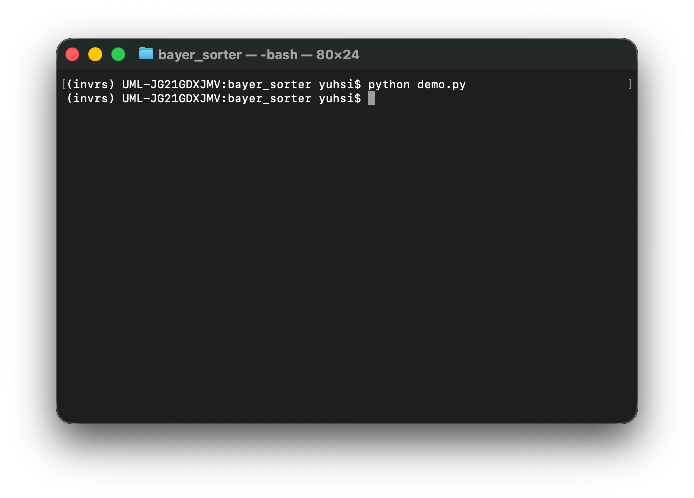

2–2. Visualize results

↪Back to the content⤴

Acknowledgments and References

• Bayer sorter
• https://github.com/invrs-io/gym
• https://github.com/invrs-io/leaderboard
• 【Reproduction】【Ubuntu 24.04.1】Bayer Sorter — Simulating Reference Design

↪Back to the content⤴