You Are Probably Clustering Your Survey Data Wrong

Encoding step nobody thinks about mattered more than the algorithm choice

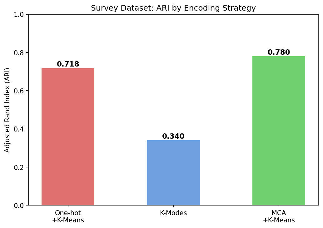
Running K-Means on a customer survey with 15 categorical questions and 5,000 respondents, gives an ARI score (calculated against ground truth) of 0.718. Then, I projected the same data through Multiple Correspondence Analysis first and ran K-Means again. With the same algorithm, same number of clusters, same random seed, ARI score increased to 0.780. The only thing that changed was how the categories were represented as numbers.

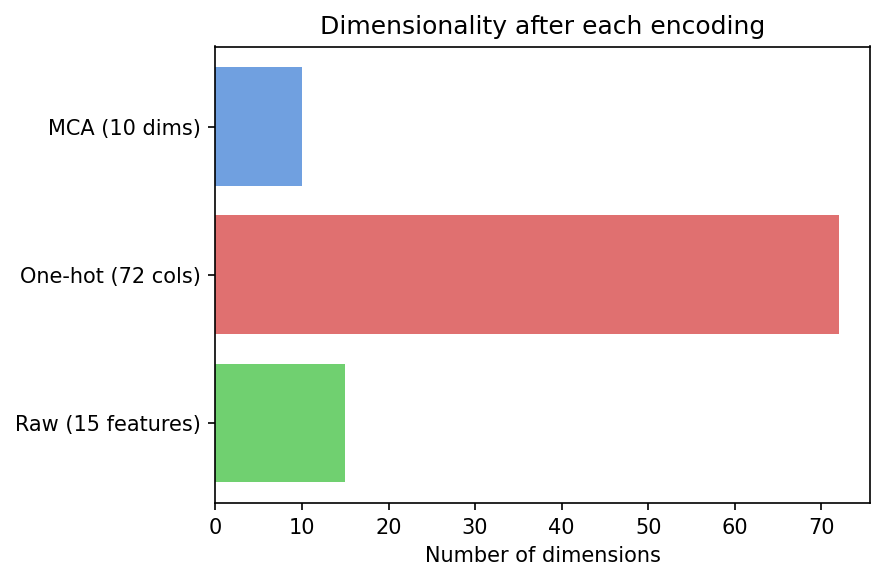
That 6-point gap comes from a problem most practitioners never check for. One-hot encoding a survey with 15 features produces 72 binary columns. Features with more answer options (product category preference with 7 options) get 7 columns. Features with fewer options (newsletter subscription with 2 options) get 2 columns. K-Means treats all 72 columns equally, which means it treats product category as 3.5 times more important than newsletter subscription. But nobody asked for that weighting.

Below, I have benchmarked five categorical clustering methods on three synthetic datasets with known ground truth. All code is available as a GitHub repository:

[embed]GitHub - Dima806/categorical_clustering_arena: A head-to-head comparison of common categorical… A head-to-head comparison of common categorical clustering methods on real-world-style datasets …github.com

Also, this article is a continuation of my other article about comparing clustering methods with numerical data:

[embed]You Are Probably Using the Wrong Clustering Algorithm K-Means lost on each of three real datasets I tested. Here is the evidencemedium.com

Let’s dive in!

Three datasets

Survey segmentation (5,000 respondents, 15 categorical features, 4 persona archetypes). Each persona has a distinct probability distribution over 15 features: preferred channel (app, online, store, phone, social), payment method (card, digital wallet, cash, bank transfer, crypto), purchase frequency (weekly through yearly), product category preference (food, electronics, clothing, home, sports, beauty, travel), and 8 more lifestyle features. Category counts range from 2 to 7 per feature.

Source: author

Customer profiles (3,000 customers, 4 categorical + 3 continuous, 3 segments). The three segments overlap on categorical features (contract type, region, acquisition channel, industry) but separate on continuous ones (monthly spend, tenure, usage frequency). This dataset tests whether methods that handle mixed types natively outperform the simple “encode everything and run K-Means” approach.

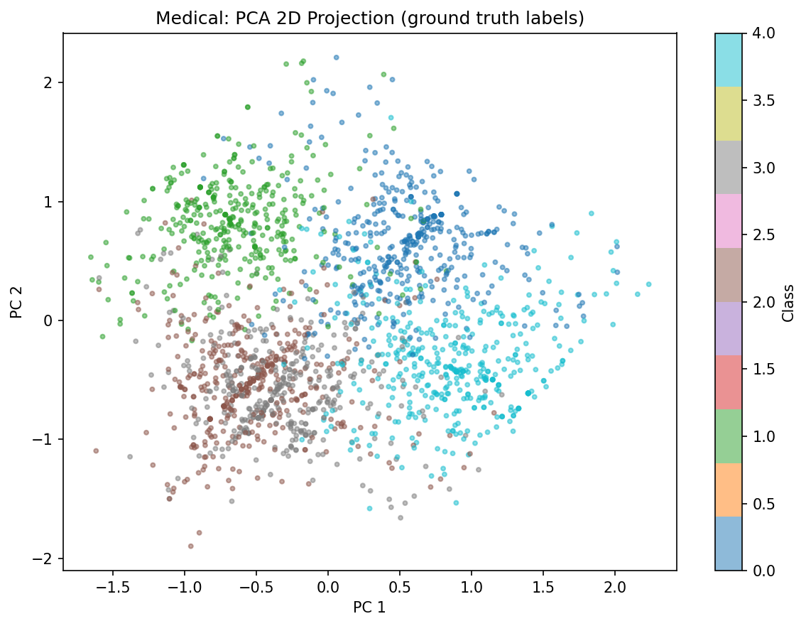
Medical symptoms (2,000 patients, 25 binary symptoms, 5 disease profiles). Twenty percent of patients have comorbidities, meaning they exhibit symptoms from two disease profiles simultaneously. This creates overlapping clusters where soft-assignment methods should have an advantage over hard-assignment ones.

One-hot problem

Most data scientists have a reflex when they get categorical data: one-hot encode it (convert each categorical feature into a set of binary columns, one per category), run K-Means (an algorithm that groups data by minimizing the distance from each point to its nearest cluster center), and report the silhouette score.

The problem is what happens to the data before the algorithm sees it. Fifteen survey features become 72 binary columns after one-hot encoding.

Source: author

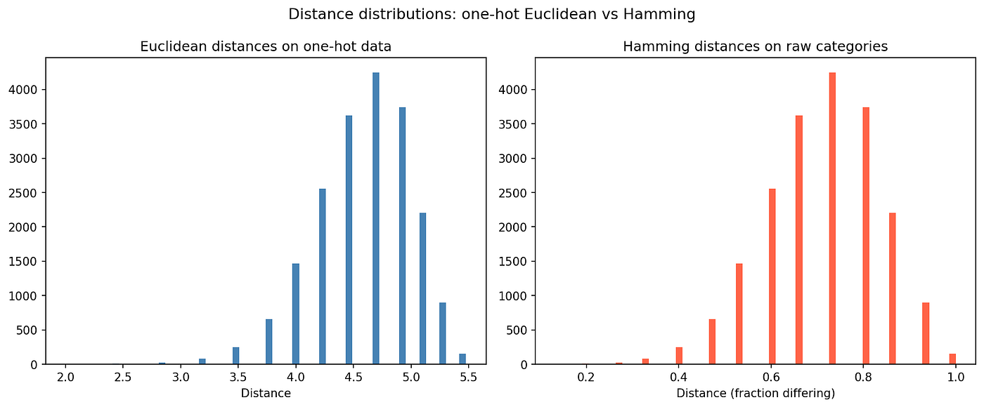
Features with more answer options carry more geometric weight. “Preferred product category” (seven options, seven binary columns) has seven times more influence on the distance than “newsletter subscription” (two options, two columns). You did not ask for that weighting. One-hot encoding imposed it.

Source: author

Hamming distance counts how many features differ between two records. Euclidean distance on one-hot data is a rescaled version of Hamming distance, but with the cardinality weighting baked in. Does this encoding difference affect the clustering?

Source: author

Yes, it does: MCA + K-Means beats one-hot K-Means by 6 ARI points using the same clustering algorithm with a different input representation.

Five clustering methods

One-hot + K-Means. The baseline: encode, cluster, done. Works when features have few categories and clusters are compact.

K-Modes. The categorical twin of K-Means. Replaces the mean centroid with the mode (most frequent category per feature per cluster) and Euclidean distance with Hamming distance. No encoding needed. In this benchmark, K-Modes used n_init=10 with Huang initialization. The low score on survey (0.340) reflects a real weakness on high-cardinality features, not bad initialization. Cao initialization might improve it, but the mode centroid fundamentally collapses the multinomial structure that LCA preserves.

LCA (Latent Class Analysis). The categorical equivalent of a Gaussian Mixture Model. Instead of fitting Gaussians, it fits a mixture of multinomial distributions (probability distributions over categorical outcomes, like the probability of each answer option on a survey question), one distribution per feature per latent class. The EM (expectation-maximization) algorithm iterates between estimating which class each record belongs to and re-estimating the class parameters until convergence. Every record gets a soft assignment: a probability of belonging to each class rather than a hard label.

from stepmix import StepMix

model = StepMix(n_components=4, measurement="categorical", random_state=42, n_init=5)
model.fit(X_encoded)
probs = model.predict_proba(X_encoded)  # shape: (n_samples, 4)

One caveat: the survey DGP generates data from a mixture of multinomials, which is exactly what LCA fits. LCA’s 8.9-point advantage over one-hot K-Means is a lower bound. On real data where the generative model is unknown and messier, LCA’s flexibility would likely matter more, and the gap could be larger.

MCA + K-Means. Multiple Correspondence Analysis (MCA) is the categorical version of PCA. It finds the axes along which survey responses vary the most, just like PCA finds the axes along which numeric measurements vary the most. Categories that frequently co-occur end up close together in the projected space. K-Means then runs on those continuous coordinates.

import prince

mca = prince.MCA(n_components=10, random_state=42).fit(X)
X_mca = mca.transform(X).to_numpy()
labels = KMeans(n_clusters=4, n_init=10, random_state=42).fit_predict(X_mca)

Gower + Hierarchical. Gower distance computes a per-feature distance (Hamming for categorical, normalized range for continuous) and averages across features. The result is a distance matrix that hierarchical clustering can use. One limitation worth noting: Ward linkage assumes Euclidean-like distances. Gower distance is not Euclidean, and using Ward on a non-Euclidean matrix can produce suboptimal merges. Average or complete linkage might be more appropriate for Gower, and the 0.448 score on survey could partly reflect this mismatch rather than a fundamental weakness of distance-based clustering.

Comparison results

Source: author

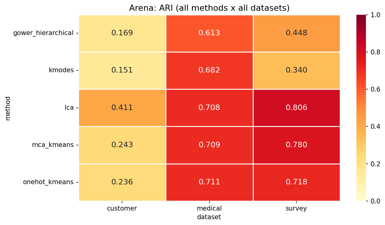
Here, LCA wins on survey, but not by the margin the literature sometimes suggests. The gap to MCA + K-Means is only 2.6 ARI points (0.807 vs 0.781). MCA is faster to fit, has no EM convergence concerns, and needs no integer re-encoding. For most production use cases, it is the better tradeoff.

On binary medical data, nothing separates the top four methods. LCA (0.708), MCA + K-Means (0.709), and one-hot K-Means (0.711) differ by less than 0.003. When features are already binary, encoding choice barely matters because one-hot encoding of a binary feature produces the same two columns that the original feature already represents.

K-Modes at 0.340 on survey is the weakest score in the comparison. Mode centroids assume clusters differ across most features simultaneously. On realistic survey data with nuanced personas that share some preferences and differ on others, that assumption breaks down.

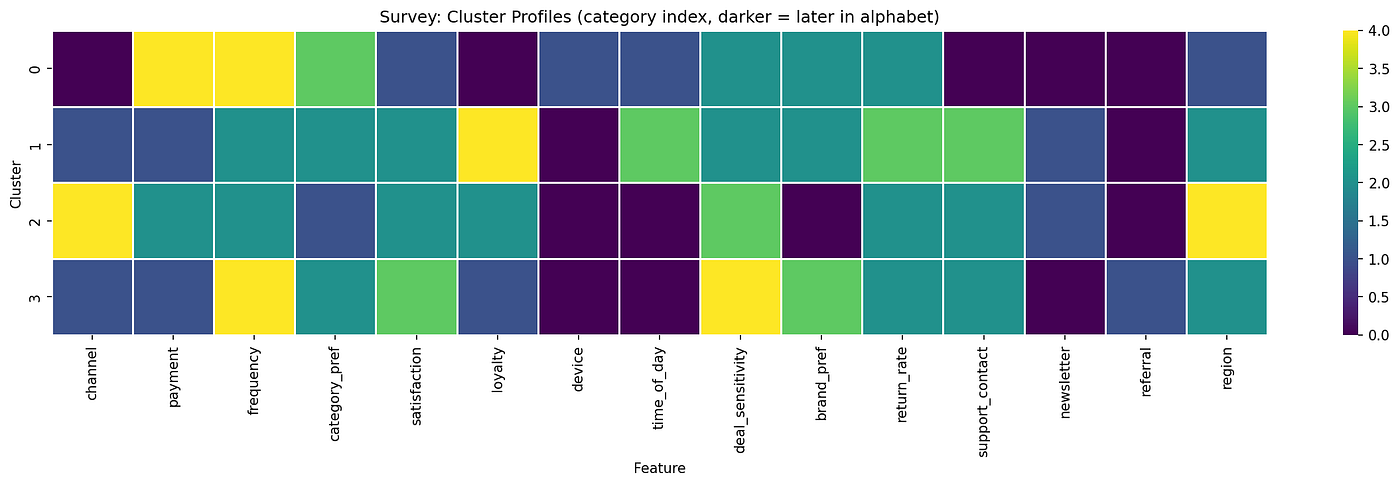
What the winning method’s output looks like in practice:

Source: author

Here, LCA produces these profiles directly from the fitted model: the class-conditional probability of each category on each feature. This is the artifact a marketing team can act on. K-Means produces centroids in one-hot space, which require manual decoding back into category names.

Mixed-data surprise

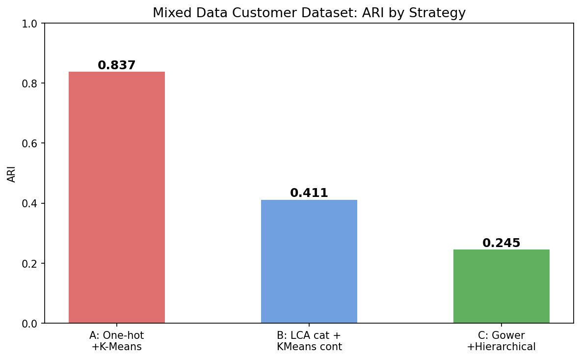
The customer dataset has both categorical and continuous features. The arena above used only categorical columns. Running all strategies on the full dataset changes the picture completely.

Source: author

One-hot encoding everything and running K-Means scores 0.837. The three continuous features (monthly spend, tenure, usage frequency) carry most of the discriminative signal. K-Means in the full standardized feature space exploits them directly. The four categorical features (contract type, region, acquisition channel, industry) add noise, but not enough to override the continuous signal.

This result is worth sitting with. A method that handles mixed types “properly” (Gower) scores 0.245. A method that ignores the type distinction entirely (one-hot K-Means on everything) scores 0.837. The difference is that Gower averages the categorical and continuous distances equally, giving the four uninformative categorical features the same total weight as the three informative continuous ones. K-Means on the standardized matrix lets the continuous features dominate naturally because their variance is higher and more cluster-discriminative.

K-Prototypes combines K-Means on continuous features and K-Modes on categorical features with a gamma weighting parameter that controls the relative importance of each type. On this dataset, gamma did nothing. ARI was 0.432 at every value from 0.1 to 10.0 because the categorical features carry so little signal that reweighting them has no effect.

The argument against one-hot encoding is real, but it applies most strongly when features are purely categorical. When you have a mix and the continuous features dominate the cluster structure, the simple approach works.

When soft assignments matter

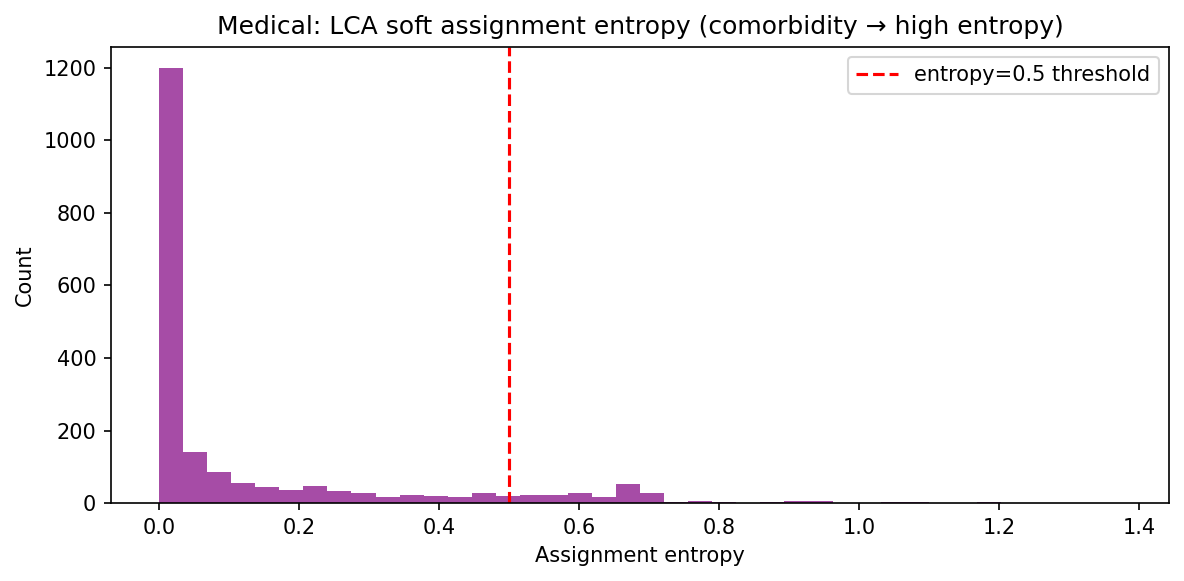
On the medical dataset, 20% of patients have comorbid symptoms from two disease profiles. LCA captures this directly.

Source: author

Entropy measures how spread out a probability distribution is. A patient assigned 99% to one class has near-zero entropy. A patient assigned 55% to class A and 40% to class C has high entropy. Consider patient 1042: LCA assigns 68% probability to profile A (respiratory), 27% to profile C (cardiovascular), and 5% spread across the rest. A hard clustering method would assign this patient to profile A and miss the cardiovascular signal entirely. LCA’s soft assignment preserves both, which matters when the downstream decision is a treatment plan that should address both conditions. The entropy histogram shows that about 8% of patients exceed the 0.5 entropy threshold, roughly matching the 20% comorbidity rate in the DGP (some comorbid patients have one dominant profile and low entropy despite having symptoms from two).

Practical guidance

For purely categorical data under 10,000 rows, start with LCA via stepmix. Use BIC (Bayesian Information Criterion), a model selection score that balances fit quality against model complexity by penalizing the number of parameters, to pick the number of classes. Fit LCA for k = 2 through 10 and choose the k where BIC is lowest. LCA gives you soft assignments and interpretable profiles that you can hand directly to a business stakeholder.

For purely categorical data above 10,000 rows, use MCA + K-Means. LCA’s EM algorithm scales linearly with n but the constant factor is larger than K-Means, and convergence can be slow with many classes. MCA + K-Means is faster and nearly as accurate. Borrow the BIC-selected k from a quick LCA run on a 5,000-row subsample, then fit K-Means on the full MCA-projected dataset.

When you have mixed categorical and continuous data, check whether the continuous features already separate your groups before reaching for a specialized method. Plot the distributions by class. If the continuous features dominate (as they did on the customer dataset, where monthly spend and tenure alone separated the three segments), one-hot everything and run K-Means on the standardized full matrix. Only reach for Gower distance when you have reason to believe the categorical features are as discriminative as the continuous ones and you can afford the O(n squared) memory cost of the full distance matrix.

For binary symptom or co-occurrence matrices, go straight to LCA. The soft assignments handle comorbid records naturally, and the class-conditional probabilities map directly to symptom profiles that clinicians can interpret.

Running it yourself

git clone https://github.com/Dima806/categorical_clustering_arena
make setup      # uv + deps, 2 CPUs / 8 GB
make test       # 55 tests, 100% coverage, ~15 sec
make notebooks  # 5 notebooks, < 5 min each
make run        # Streamlit app on :8501

Drop your questions in the comments below 😊