🧠 Deciphering the Model’s Memory: Mutual Information and the Code-Length of Data

In Part 1, we introduced the idea that language models can “memorize” parts of their training data — sometimes harmlessly, sometimes in ways that create privacy risks.

But how do researchers actually measure memorization?

This paper introduces a remarkably elegant answer using two ideas from information theory and computer science:

1. Mutual Information (MI) — how much two things “know” about each other.
2. Kolmogorov Complexity (KC) — how hard something is to describe or compress.

Together, these ideas turn memorization into something measurable in bits (a measurable, auditable score).

The Core Intuition

Imagine training a language model on millions of sentences. After training, the model’s parameters (its weights) contain some information about the dataset. The central question becomes:

“How much does knowing the trained model help us reconstruct a specific training example?”

If knowing the model makes a training example much easier to predict, then the model likely memorized it. If the model only learned general language patterns, then knowing the model helps only a little.

This idea is exactly what Mutual Information measures.

The Currency of Information: Bits and Tokens

Before we tackle the big concepts, let’s establish the unit of measurement. In information theory, everything is measured in bits.

• Information Content (Self-Information): This concept quantifies the “surprise” of an event. A very rare event is highly surprising and carries a lot of information; a very common event is not surprising and carries little information. Mathematically, for an event with probability P(x), the information content is:

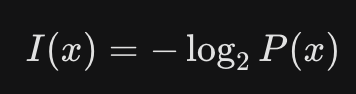
• The base of the logarithm, log_2, ensures the unit is the bit. For LLMs, a sequence of tokens (sub-words or characters) is the data unit. The likelihood a model assigns to a token sequence directly relates to the information content (or “surprise”) of that sequence.

Mutual Information: Quantifying Shared Knowledge

Mutual Information is the central metric that answers: How much does knowing the model’s brain (θ) help us predict a specific piece of training data (x_i)?

Mutual Information measures: How much knowing one thing reduces uncertainty about another thing.

Mathematically: [I(X;Y)] means: “How much information is shared between X and Y?”

Intuition with Examples

Example 1 — No Shared Information

Suppose:

• X = outcome of rolling one dice
• Y = today’s weather

Knowing the weather tells you nothing about the dice roll.

So: [I(X;Y) ~ 0]: No mutual information.

Example 2 — Strong Shared Information

Suppose:

• X = exam answers
• Y = leaked answer sheet

Now knowing Y almost fully reveals X.

Mutual Information becomes very high.

What is Mutual Information (MI)?

Mutual Information I(X; Y) is a measure of the mutual dependence between two random variables, X and Y. It quantifies the reduction in uncertainty about one variable given knowledge of the other.

MI = 0: The variables are independent (knowing Y tells you nothing about X).

MI = High: The variables are highly dependent (knowing Y significantly reduces your uncertainty about X).

What Are the Two Variables Here (Calculating Memorization via MI)?

In this context of the paper, the two random variables are:

1. The Training Data Point (X) = a training data point (x_i); a specific example x_i from the dataset (e.g., a sentence or a private code snippet).
2. The Model’s Parameters (θ) = the trained model parameters; the entire set of weights and biases θ learned by the LLM.

So the paper studies:

[I(x_i ; θ)] Meaning: “How much does knowing the model’s parameters reduce uncertainty about a specific training example?”

The memorization score for a data point x_i is equivalent to estimating the mutual information I(x_i; θ).

This works because:

• High Memorization → The data point x_i is highly correlated with the final parameters θ. Knowing θ makes x_i extremely predictable (low uncertainty).
• Low Memorization (Generalization) → The data point x_i contributed to general patterns, but its exact sequence is not stored. Knowing θ helps a little (it’s a correct English sentence), but doesn’t make it perfectly predictable.

The Uncomputable Ideal: Kolmogorov Complexity

To calculate MI for memorization, the researchers use a formulation that relates to Kolmogorov Complexity (K).

What is Kolmogorov Complexity (K(x))?

Kolmogorov complexity K(x) is the length of the shortest possible computer program (in a fixed programming language) that can generate a data string x. It is the ultimate measure of a string’s algorithmic information content or its inherent non-redundancy.

• Low K(x): The string has a simple pattern and is highly compressible (e.g., “AAAAA…” can be generated by a short program: ‘Print “A” 100 times’).
• High K(x): The string appears random and cannot be compressed (e.g., a random sequence of characters).

Connecting K(x) to Memorization

The formula for the memorization score of a data point x_i given the model θ is:

This equation captures the intuition that memorization is the compression achieved by the model.

• K(x_i): The inherent complexity of the data point without knowing the model. This is the raw information content.
• K(x_i | θ): The complexity of the data point after knowing the model’s parameters. This is the remaining uncertainty/surprise about x_i.
• If the model memorized x_i verbatim: The model’s parameters θ encode the exact sequence. When you try to describe x_i given θ, the description can be very short (e.g., “just output the thing you memorized”). Thus, K(x_i | θ) is very small. The gap, K(x_i) — K(x_i | θ), is large, indicating high memorization.
• If the model generalized x_i: θ only encodes the general rules (English grammar) that generated x_i, not the specific sequence. K(x_i | θ) remains close to K(x_i), as the model doesn’t save much on the description length. The gap is small, indicating low memorization.

The Practical Workaround: Approximating with Negative Log-Probability

A key challenge is that Kolmogorov Complexity K(x) is mathematically uncomputable. You can never guarantee you’ve found the absolute shortest program.

The paper solves this by using the most effective tool available to estimate information content: the Negative Log-Likelihood (NLL), which is directly related to the concept of surprisal or information content we discussed earlier.

NLL as an Information-Theoretic Proxy

For any data point x_i and a probability distribution P (or an LLM’s predictive distribution Pθ), the NLL is:

This is an approximation of K(x_i), where the “program” is implicitly the probability model used to describe the data.

The paper, therefore, approximates the difference in Kolmogorov complexity with the difference in negative log-probabilities (or “surprisal”):

Here, Pθ(x_i) is the probability the trained LLM θ assigns to the sequence x_i, and Pprior(x_i) is the probability assigned by a simple, untrained “prior” model (like a random guess or a basic compression algorithm).

The final memorization score Mem(x_i | θ) is practically calculated by:

Example: The Random Sequence

• Training Example: flornix zabello prentak (a rare, random sequence repeated 100 times in training).
• Prior Model Pprior(x_i): The sequence is highly random, so Pprior(x_i) is very low. Initial Surprise -log(Pprior(x_i)) is Very High.
• Trained LLM Pθ(x_i): The LLM has memorized the sequence. It predicts each token with near-perfect confidence. Pθ(x_i) is very high. Remaining Surprise is Very Low.
• Result: A Large Memorization Score, as the model dramatically reduced the surprise (i.e., compressed it).

This quantitative framework allows us to not only say a model memorized data, but to measure how many bits of information it retained from that specific training example, giving developers a precise tool for privacy audits.

For a clearer visual explanation of the relationship between two variables that can be measured with mutual information, you can watch this video.

Mutual Information, Clearly Explained!!!