Mesa: Operational Framework for High-Fidelity Agent-Based Modeling

1. Executive Logic: The Foundation of Agent-Based Simulations

In the architecture of complex systems, the strategic importance of execution logic cannot be overstated. Agent-based models (ABM) are predicated on the emergence of system-level behaviors from individual entities following localized rules. For these emergent patterns to be scientifically valid, a rigorous operational framework is essential. Without it, the scaling of entity-level rules into system-wide phenomena risks being undermined by computational artifacts rather than true logic.

The Anatomy of the Modeling Framework

A professional simulation environment is built upon a three-pillar architecture derived from the Mesa framework:

1. Modeling: The foundational layer consisting of agent classes, spatial environments, and the core model class. This layer handles the internal state and the mechanics of interaction.
2. Analysis: The diagnostic suite used to aggregate data from simulation runs, allowing for sensitivity analysis across varying parameter sets.
3. Visualization: The interface layer — specifically browser-based — enabling real-time monitoring and visual validation of model behaviors.

The Role of Modeling Modules

Modeling modules are the direct drivers of the system state. They define the interplay between agent properties and the spatial parameters they inhabit. In this framework, agents are not static; they possess internal state variables, such as age, which evolve as the simulation progresses. The modeling modules ensure that as the simulation iterates, these state changes are recorded and governed by the predefined rules of the environment, transforming abstract code into a functioning, dynamic system.

import mesa

class MyAgent(mesa.Agent):
 def init(self, model, age):
  super().init(model)
  self.age = age
 def step(self):
    self.age += 1
    print(f"Agent {self.unique_id} now is {self.age} years old")
    # Whatever else the agent does when activated

class MyModel(mesa.Model):
 def init(self, n_agents):
  super().init()
  self.grid = mesa.discrete_space.OrthogonalMooreGrid((10, 10), torus=True)
  initial_ages = self.rng.integers(0, 80, size=n_agents)
  agents = MyAgent.create_agents(self, n_agents, initial_ages)
  for agent in agents:
  agent.cell = self.grid.all_cells.select_random_cell()
 def step(self):
    self.agents.shuffle_do("step")

Operational Objective

The primary objective of this framework is to transform decentralized agent rules into structured, reproducible system insights. By standardizing population management and temporal progression, the framework ensures that results are the product of intended logic. This rigorous approach bridges the gap between abstract theoretical modeling and the rigid physical constraints of the simulated environment.

2. Spatial Architecture: Configuring Discrete and Continuous Environments

Spatial configuration serves as the “physics” of the simulation. The choice of space is a functional determinant of agent proximity, connectivity, and interaction frequency. Selecting a spatial environment is a strategic decision that dictates how agents perceive and navigate their world.

Discrete Grid Environments

The Orthogonal Von Neumann Grid is a primary choice for discrete modeling. In this configuration, connectivity is strictly limited to four directions: up, down, left, and right. By excluding diagonals, the architect imposes specific interaction constraints that are vital for simulating structured environments like urban layouts or cellular automata.

• Torus Configuration: This setting enables the grid to wrap at the edges (Pac-Man style). An agent exiting the right boundary reappears on the left, which is essential for simulating continuous surfaces without the distortion of “edge effects.”
• Fixed-Boundary Grids: When torus=False, edges act as hard physical boundaries. Agents are confined within the grid limits, a requirement for modeling geographically or structurally constrained systems.

Relational Topologies (Network Space)

In Network Space, the focus shifts from physical coordinates to graph theory. Agents exist on nodes, and their interactions are governed solely by the defined edges (connections) between them. This topology is the gold standard for modeling social dynamics, supply chains, or infrastructure where relational proximity outweighs physical distance.

Irregular Tessellation (Voronoi Space)

Voronoi Space utilizes a Voronoi mesh to create an irregular tessellation. Unlike uniform grids, the mesh divides space based on the proximity to a set of center points. This creates a coordinate-independent structure where “territory” is a function of point density. It is superior for simulating natural resource competition or territories that do not conform to rigid squares.

Continuous Space vs. Discrete Space

While discrete spaces use cells or nodes, Continuous Space allows for precise, coordinate-based movement. This is vital for high-fidelity physical modeling where the constraints of a grid would introduce unwanted discretization errors in agent trajectory and positioning.

Comparison of Spatial Environments

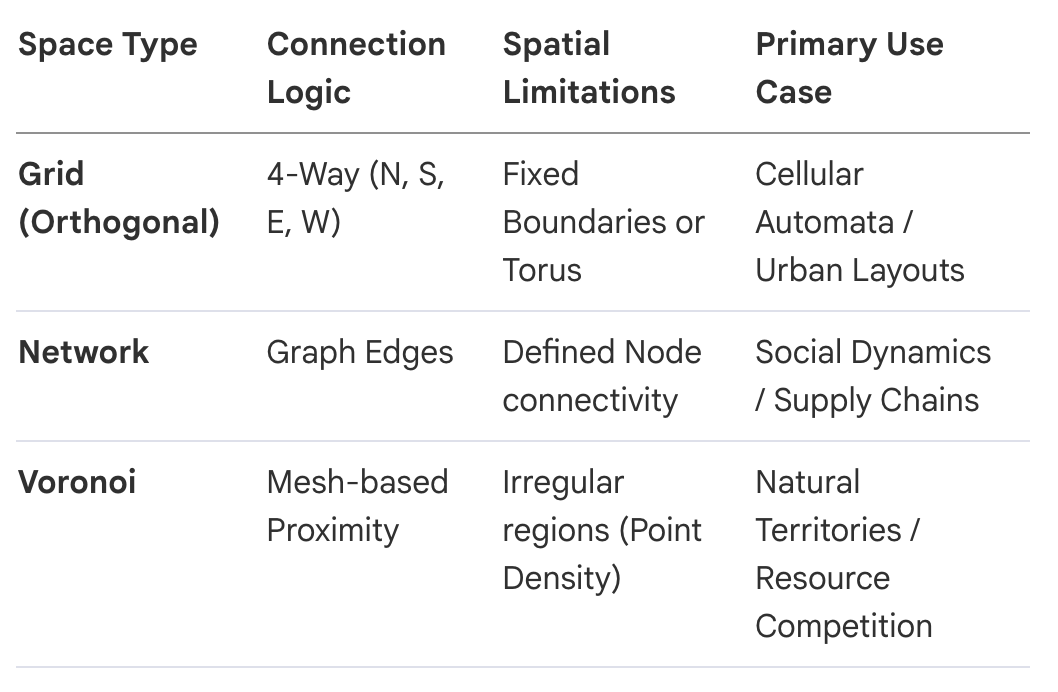
As these spatial parameters define the “where,” the population’s “who” is managed through dynamic AgentSets.

3. AgentSet Management: Dynamic Population Control

The AgentSet is the central management tool for maintaining simulation fidelity. It functions as a dynamic container that is automatically updated whenever agents are added or removed from the model. This automation ensures that the simulation state remains stable and reflective of the current population without requiring manual registry management.

Functional Capabilities of AgentSets

• Selection & Filtering: Isolate agents based on specific state criteria to ensure logic is applied only to relevant entities.
• Shuffling & Sorting: Randomize or order agents by attributes to eliminate execution bias.
• Method Application: Broadcast commands (e.g., step or move) across the entire set or a filtered subset with high efficiency.

Macro-Level Metrics from Micro-Level Interactions

AgentSets provide built-in statistical aggregation tools (mean, sum, etc.). These are critical for deriving macro-level metrics from individual agent attributes. For instance, calculating the average age across an AgentSet allows the architect to observe population-wide trends emerging from individual lifecycle rules.

Primary AgentSet Functions

• Selecting: It ensures targeted logic application by isolating agents that meet specific simulation requirements.
• Shuffling/Sorting: It eliminates “order-of-execution” bias, ensuring results aren’t skewed by the sequence of agent creation.
• Applying Methods: It enables efficient, mass-execution of behaviors across the population via a single architectural command.
• Aggregating: It transforms micro-data into high-level metrics required for system-wide analysis and reporting.
• Grouping: It allows for the comparative analysis of distinct sub-populations based on shared attribute values.

4. Scheduling Protocols and Activation Cycles

In a computational simulation, true simultaneity is an illusion. The sequence of agent actions is as critical as the actions themselves. Robust scheduling prevents simulation artifacts where one agent’s action unfairly invalidates another’s within the same time step.

Temporal Units

The simulation progresses in discrete units. By default, each model.step() represents exactly 1.0 time units. This technical consistency ensures that a command like run_for(10) executes precisely 10 steps, maintaining temporal alignment across different simulation runs.

Sequential vs. Random Activation

Sequential activation carries a high risk of ordering bias. To maintain high fidelity, the architect utilizes the **shuffle_do** method. By randomizing the activation order at every step, the framework ensures that no single agent is consistently prioritized in resource acquisition or movement.

Multi-Stage Activation Cycles

Complex models require partitioning behaviors into distinct stages across the population: move ➡️ eat ➡️ reproduce. This partitioning is a requirement to avoid simultaneous state-change conflicts. For example, it prevents two agents from “eating” the same resource in a single step by ensuring all movement is resolved before any consumption logic begins.

Activation Checklist

• Sequential: Use only when a specific, fixed hierarchy of action is a functional requirement of the model.
• Random (shuffle_do): Use as the mandatory default for most interactions to mitigate ordering bias.
• Multi-stage: Use when distinct behaviors must be synchronized across the whole population to prevent state conflicts.
• Type-based: Use for models with specialized classes (e.g., Predators and Prey) that require differentiated execution logic.

5. Analysis and Visualization: From Simulation to Insight

The terminal phase of the framework focuses on the extraction of actionable data and the visual validation of emergent behaviors. A simulation is only as useful as the insights it generates and the confidence stakeholders have in its execution.

Verification and Data Collection

Analysis modules gather data across multiple runs, allowing for the observation of system sensitivity to parameter shifts. Simultaneously, the browser-based visualization interface provides real-time monitoring. For a Simulation Architect, this is not just aesthetic; it allows for the real-time visual verification of property increments (such as age) and spatial distributions, ensuring the model's logic is behaving as intended.

Best Practices for High-Fidelity Modeling

1. Eliminate Ordering Bias: Default to shuffle_do for agent activation unless a fixed hierarchy is mathematically necessary.
2. Standardize Temporal Increments: Maintain the 1.0 time unit per step to ensure comparability across simulation batches.
3. Align Space with Logic: Select the spatial environment (Grid, Network, or Voronoi) based on the relational physics of the real-world system.
4. Prevent State Conflicts: Utilize multi-stage activation cycles to partition behaviors and maintain logical consistency.
5. Monitor Micro-Macro Links: Use AgentSet aggregation tools to track population-level metrics in real-time to catch anomalies early.

The integrity of any complex system simulation rests upon the synergy between spatial constraints and temporal scheduling. By adhering to this integrated operational framework, practitioners can ensure that emergent behaviors are a true reflection of system logic, providing a professional foundation for scientific and operational insight.

https://mesa.readthedocs.io/latest/overview.html