How Transformers Become Faster And Smarter: From KV Cache to MLA

Explore the fundamental evolution of the LLM decoder inference

Today, Transformers have become the basic paradigm of LLM and basic AI models. Now, Transformer is not only chatting with you, but also solving your real problem. It needs to understand more context of your question, for example, reading the 900 pages of *OBBBA* to tell the possible impact on your business, or understanding the 100K lines of code to fix a hidden bug in your software.

source: generated by GPT-5. I asked it to generate a cover image for my article.

However, the input size of those models is limited, and the long-context input and reasoning become the real practical technical challenge that can truly impact the AI industry.

There are many technical directions to tackle the long-context problem. This article tries to dig into one of them: The KV Cache optimization.

The QKV in Salf-Attention

We have introduced the Self-Attention (SA) in “*The Great Transformer”, which is the key mechanism of Transformers. In the SA, Each input token, which practically represents a word/pixel/concept in the Large Language Model (LLM), would be projected to 3 vectors: Query, Key, and Value* (QKV), which are the inputs of the SA algorithm.

Source: KV Cache Explained Intuitively

When we add more tokens, which means we are adding words/pixels/concepts to the AI model, the token will be extended from a vector to a matrix. The new token would be added to the last row of the matrix.

For example, when we add tokens from 1 to 3, it would be like:

Source: KV Cache Explained Intuitively

Even though the softmax computation is the bottleneck of the computation, the computation from token to Q/K/V is also heavy, especially in the decoder.

Decoder Inference

Assume your LLM has L layers, and the length of your output is N, then the simplified inference procedure of your decoder is:

1. Feed the input X(length=1) to L layers. Each layer generates 1 vector for QKV. The decoder generates one token y₁.
2. Concatenate the y₁ to the input X, and feed the input X(length=2) to L layers. Each layer generates 2 vectors for QKV. The decoder generates one token y₂.
3. Concatenate the y₂ to the input X, and feed the input X(length=3) to L layers. Each layer generates 2 vectors for QKV. The decoder generates one token y₃.
4. Repeat…
5. Concatenate the yₙ₋₁ to the input X, and feed the input X(length=n) to L layers. Each layer generates n vectors for QKV. The decoder generates one token yₙ.

The decoder runs multiple times to decode every single word. Source: The Illustrated Transformer

The problem with the procedure is that we need to compute the QKV for L ×(1 + 2 +…+ N) times. It’s an O(N²) complexity. The good news is, we can reduce the complexity by caching.

KV Cache

If we look into the SA formula, each token position, which means each row in the Q, K, V, and the output(Z) metrics, is relevant to every other position. That’s how self-attention design.

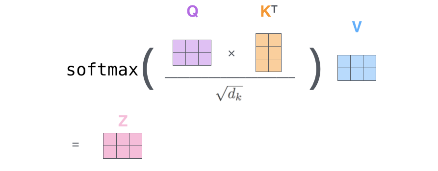
The self-attention calculation in matrix form. Source: The Illustrated Transformer

But in the decoder, each row of Q, K, and V is only relevant to its history, not the future. A.k.a, the autoregression. So the LLM decoder designs a *causal mask inside the softmax to mask out the future. In this case, the i-th row of Q, K, and V is only relevant to the rows that are less than the i-th* row.

To do it, we can just concatenate the i-th key (i-th row in K) and value (i-th row in V) at the bottom of the current (i-1)-th K and V.

To experiment that the concatenation didn’t break the value or math in the SA layers in the decoder, I wrote the following Python experiments:

import torch
import math
import matplotlib.pyplot as plt

torch.set_printoptions(precision=6, sci_mode=False)
# ----- Hyperparameters -----
seed = 0
torch.manual_seed(seed)
d_model = 1   # single value (1x1) as requested
d_k = 1       # single-head attention with 1-dim projections
L = 3         # number of layers
T = 5         # context length to grow to
d_ff = 4      # hidden size for the feed-forward layer
dtype = torch.float64
device = torch.device("cpu")
# ----- Random weights and initial token -----
WQ = torch.randn(d_model, d_k, dtype=dtype, device=device)
WK = torch.randn(d_model, d_k, dtype=dtype, device=device)
WV = torch.randn(d_model, d_k, dtype=dtype, device=device)
# Feed-forward layer weights (shared across layers)
W1 = torch.randn(d_k, d_ff, dtype=dtype, device=device)
W2 = torch.randn(d_ff, d_model, dtype=dtype, device=device)
X = torch.randn(1, d_model, dtype=dtype, device=device)  # initial (1x1)

def causal_self_attention(X):
    """
    X: (t, d_model)
    Returns: (out, Q, K, V, attn)
    """
    Q = X @ WQ  # (t, d_k)
    K = X @ WK  # (t, d_k)
    V = X @ WV  # (t, d_k)
    t = X.size(0)
    scores = (Q @ K.T) / math.sqrt(d_k)  # (t, t)
    mask = torch.triu(torch.ones(t, t, dtype=torch.bool, device=X.device), diagonal=1)
    scores = scores.masked_fill(mask, -1e9)
    attn = torch.softmax(scores, dim=-1)  # (t, t)
    out = attn @ V                        # (t, d_k)
    return out, Q, K, V, attn, mask

def feed_forward(X):
    """Position-wise feed-forward: ReLU(X @ W1) @ W2
    X: (t, d_k) -> (t, d_model)
    """
    return torch.relu(X @ W1) @ W2
print("=== Weights ===")
print("WQ:", WQ.view(-1))
print("WK:", WK.view(-1))
print("WV:", WV.view(-1))
print("W1:", W1.view(-1))
print("W2:", W2.view(-1))
print("\nInitial X (t=1):", X.view(-1))
for t in range(1, T + 1):
    X_l = X
    Ks, Vs, Qs = [], [], []
    # Apply the SAME SA L times (L identical layers), followed by FF each time
    for l in range(L):
        Z, Q, K, V, attn, mask = causal_self_attention(X_l)
        # Feed-forward layer after self-attention
        X_l = feed_forward(Z)  # (t, d_model) -> next layer input
    # Report (use the last layer to keep output compact)
    print(f"\n=== Step t={t} (sequence length {X.size(0)}) ===")
    print(f"K (layer {L}) shape={tuple(K.shape)}:\n{K.view(-1)}")
    print(f"V (layer {L}) shape={tuple(V.shape)}:\n{V.view(-1)}")
    print(f"Q (layer {L}) shape={tuple(Q.shape)}:\n{Q.view(-1)}")
    print(f"Z (layer {L}) shape={tuple(Z.shape)}:\n{Z.view(-1)}")
    # ----- Visualization -----
    fig, axs = plt.subplots(1, 3, figsize=(15, 5))
    # Q, K, V bar plots
    axs[0].bar(range(Q.shape[0]), Q.view(-1).cpu().numpy(), label="Q")
    axs[0].set_title('Q')
    axs[1].bar(range(K.shape[0]), K.view(-1).cpu().numpy(), label="K", color='orange')
    axs[1].set_title('K')
    axs[2].bar(range(V.shape[0]), V.view(-1).cpu().numpy(), label="V", color='green')
    axs[2].set_title('V')
    # Mask as image
    # Create a new figure for mask and attn if t > 3 to prevent small images
    fig2, axs2 = plt.subplots(1, 2, figsize=(8, 4))
    axs2[0].imshow(mask.cpu().numpy(), cmap='gray', vmin=0, vmax=1)
    axs2[0].set_title('Mask')
    axs2[1].imshow(attn.detach().cpu().numpy(), cmap='viridis')
    axs2[1].set_title('Attention')
    plt.tight_layout()
    plt.show()
    # Grow sequence by appending the LAST token of the final layer's output
    if t < T:
        new_token = X_l[-1:].detach()   # (1, d_model)
        X = torch.cat([X, new_token], dim=0)
print("\nDone. Observation: For every t>1 and for every layer, the first t-1 rows of K and V "
      "are exactly equal to those computed at t-1. Hence, KV is cacheable.")

Here’s the output:

1st layer

2nd layer

3rd layer

4th layer

5th layer

So actually, we don’t need to recompute the old K and V, but only cache the history K and V and concatenate the new vector k and v to them. This will reduce the time complexity from O(N²) to O(N). We call it KV cache.

Why do we only cache the K and V but not Q, even though the V is also a causal mask? Because the i-th output is only relevant to the matrices Q and V, and the i-th query vector. So caching the past Q matrix is meaningless because we don’t need it afterward.

Source: KV Cache Secrets: Boost LLM Inference Efficiency

But can we be faster? We’ve done the self-attention layer, now we can try something on the MHA, multi-head attention.

MQA and GQA

To make it faster, we need to compress the information. In the MHA, we have multiple branches, which we call “heads”, of the self-attention blocks, and merge them afterward. Each head has its own Q, K, and V metrics. Here comes a straightforward solution: sharing the K and V.

Source: GQA: Training Generalized Multi-Query Transformer Models from Multi-Head Checkpoints

Each column in the illustration represents a “head”. The leftmost multi-head attention shows that each head has its one Q, K, and V.

The Multi-Query Attention, MQA, in the rightmost column, is the wildest approach that shares the K and V across the heads. The MQA saves the most memory and projection computation, but also unavoidably drops the accuracy of the model because it compresses the K/V information across the heads.

The Grouped-Query Attention, *GQA, in the middle, is a simple and elegant paper proposed by Google Research in 2023. Some heads are sharing a common V and K, but keep their own queries. This makes a good balance between MHA and MQA that keeps the minimal accuracy drop from MHA, but the inference time is very close to MQA. The following illustration shows the speed-accuracy trade-off between MHA, MQA, and GQA*.

Source: GQA: Training Generalized Multi-Query Transformer Models from Multi-Head Checkpoints

BTW, the reason why they only share the K and V but not Q is that if they share 3 of them, then their output would also be identical, which loses the meaning of multi-head.

Google makes the K/V computation simpler, but the DeepSeek cracks it deeper.

The Multi-Latent Attention, MLA

In the MHA decoder with KV cache, the time complexity for projecting each input token to Q, K, and V is O(H×L️×dₖ×d), where H is the number of heads, L is the length of input so far, and dₖ is the dimension of each column in Q/K/V, and d is the dimension of the input token.

With MQA or GQA, it can be faster by reducing redundant computation or data compression, but the time complexity doesn’t change because the projection of V is inevitable.

The MLA, Multi-Latent Attention, proposed in the *DeepSeek V2, solves this by projecting the K/V to a latent space with dimension r, and let r ≪ dₖ. When we perform linear projection from dimension d to dₖ*, we can project it to a lower-dimensional space and reproject it to a higher-dimensional space.

Source: DeepSeek V2 paper

For example, if we project from the d-dimensional input token to the dₖ-dimensional vector, the computation time is dₖ×d. But if we project it to another dimension r and reproject it to dₖ, the computation time becomes (d×r) + (dₖ×r).

If dₖ=100, d=100, and r=20, then the original computation time is dₖ×d=10000, and the computation time with reprojection is (d×r) + (dₖ×r)=2000+2000=4000, which improved 60%.

It’s not a new trick. It’s mathematically similar to the *1×1 convolution idea from a decade ago by [GoogleNet](https://arxiv.org/abs/1409.4842). However, the purpose of it in the LLM era is different than what it was in the CNN era. In the CNN* era, we can put our model on one GPU, the bottleneck is the inference time. But in the LLM era, the model is too big to put into a GPU, so the memory became the bottleneck.

In the original KV cache, we keep the dₖ-rank KV cache in memory for thousands of heads and input lengths. But with the MLA, we only need to cache the r-rank compressed cache in the memory, where r is set to be far less than dₖ, so we can save more memory to more heads or deeper layers. According to the *DeepSeek V2 paper, the computation cost of MLA is similar to that of GQA with 2.25 groups, but the accuracy is much better than GQA. Overall, the MLA reduces 93.3% KV cache of the original 67B model*.

Source: DeepSeek V2 paper

Summary

From the first time we tried ChatGPT, we were very frustrated by its slow text generation. But nowadays, nobody is complaining about the throughput anymore because what’s beyond the LLM, the MHA computation, has been boosted a lot; the KV Cache in this article is just a branch of it.

KV cache has always been an important algorithm for LLM, either in system engineering or algorithm optimization. From now on, MLA has just implemented the 1x1 convolution to KV cache, which was almost 10 years ago, and it makes me believe that we still have lots of work from the past decade that could apply to LLM. Most likely, the LLM could definitely be faster in the future.