Understanding and Implementing the Wald Test in R
The Wald test is a fundamental statistical tool used to test hypotheses about parameters in a model. In R programming, it is beneficial for…
Understanding and Implementing the Wald Test in R
The Wald test is a fundamental statistical tool used to test hypotheses about parameters in a model. In R programming, it is beneficial for evaluating the significance of coefficients in linear and generalized linear models. This article delves into the intricacies of the Wald test in R, providing a comprehensive guide on its implementation, interpretation, and practical applications. Whether you’re a seasoned data analyst or a novice, this guide will equip you with the knowledge and skills to effectively utilize the Wald test in your data analysis projects.
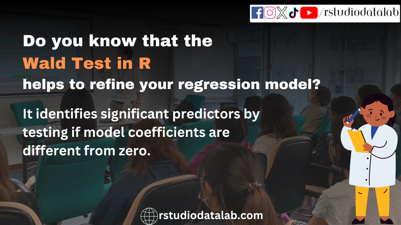
Read the complete article and also get a code: Wald Test in R
What is the Wald Test?
The Wald test is a statistical test used to evaluate the significance of parameters in a model. It is based on the Wald statistic, which measures the difference between the estimated parameter and its hypothesized value relative to the standard error of the estimate. The test is beneficial in regression analysis, which helps determine whether a particular coefficient significantly differs from zero.
In R, the Wald test can be performed using the Wald.test function from the aod package. This function allows you to test hypotheses about the coefficients of a linear model, providing a robust way to assess the significance of predictors.
https://open.spotify.com/episode/5C4oxBVZ0mhVFZj5jQQnSM/embed
Why Use the Wald Test?
The Wald test offers several advantages over other hypothesis testing methods. Firstly, it is computationally efficient and straightforward to implement. Secondly, it provides a clear and interpretable measure of the significance of model parameters. The Wald test can also be applied to many models, including linear regression, logistic regression, and generalized linear models.
However, the Wald test has its limitations. It assumes that the sample size is sufficiently large and that the model is correctly specified. Violations of these assumptions can lead to inaccurate results. Despite these limitations, the Wald test remains valuable in the data analyst’s toolkit.
When to Use the Wald Test
The Wald test is typically used in the following scenarios:
- Testing the Significance of Individual Coefficients: To determine whether a particular predictor significantly affects the outcome variable.
- Comparing Nested Models: To compare the fit of nested models and assess the significance of additional predictors.
- Hypothesis Testing in Generalized Linear Models: To test hypotheses about the parameters in generalized linear models, such as logisticregression.
How to Perform the Wald Test in R
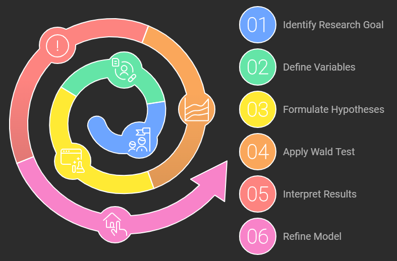
Performing the Wald test in R involves several steps, including fitting a model, extracting the coefficients and their variance-covariance matrix, and applying the wald.test function. Below is a step-by-step guide to performing the Wald test in R.
Step 1: Install and Load Required Packages
Before performing the Wald test, you must install and load the necessary packages. The aod, sandwich, and lmtest packages are commonly used.
Step 2: Fit a Linear Model
The first step in performing the Wald test is to fit a linear model to your data. For this example, we will use the mtcars dataset built into R.
##       mpg             cyl             disp             hp
##  Min.   :10.40   Min.   :4.000   Min.   : 71.1   Min.   : 52.0
##  1st Qu.:15.43   1st Qu.:4.000   1st Qu.:120.8   1st Qu.: 96.5
##  Median :19.20   Median :6.000   Median :196.3   Median :123.0
##  Mean   :20.09   Mean   :6.188   Mean   :230.7   Mean   :146.7
##  3rd Qu.:22.80   3rd Qu.:8.000   3rd Qu.:326.0   3rd Qu.:180.0
##  Max.   :33.90   Max.   :8.000   Max.   :472.0   Max.   :335.0
##       drat             wt             qsec             vs
##  Min.   :2.760   Min.   :1.513   Min.   :14.50   Min.   :0.0000
##  1st Qu.:3.080   1st Qu.:2.581   1st Qu.:16.89   1st Qu.:0.0000
##  Median :3.695   Median :3.325   Median :17.71   Median :0.0000
##  Mean   :3.597   Mean   :3.217   Mean   :17.85   Mean   :0.4375
##  3rd Qu.:3.920   3rd Qu.:3.610   3rd Qu.:18.90   3rd Qu.:1.0000
##  Max.   :4.930   Max.   :5.424   Max.   :22.90   Max.   :1.0000
##        am              gear            carb
##  Min.   :0.0000   Min.   :3.000   Min.   :1.000
##  1st Qu.:0.0000   1st Qu.:3.000   1st Qu.:2.000
##  Median :0.0000   Median :4.000   Median :2.000
##  Mean   :0.4062   Mean   :3.688   Mean   :2.812
##  3rd Qu.:1.0000   3rd Qu.:4.000   3rd Qu.:4.000
##  Max.   :1.0000   Max.   :5.000   Max.   :8.000
##
## Call:
## lm(formula = mpg ~ hp + wt, data = mtcars)
##
## Residuals:
## Min 1Q Median 3Q Max
## -3.941 -1.600 -0.182 1.050 5.854
##
## Coefficients:
## Estimate Std. Error t value Pr(>|t|)
## (Intercept) 37.22727 1.59879 23.285 < 2e-16 ***
## hp -0.03177 0.00903 -3.519 0.00145 **
## wt -3.87783 0.63273 -6.129 1.12e-06 ***
## ---
## Signif. codes: 0 '***' 0.001 '**' 0.01 '*' 0.05 '.' 0.1 ' ' 1
##
## Residual standard error: 2.593 on 29 degrees of freedom
## Multiple R-squared: 0.8268, Adjusted R-squared: 0.8148
## F-statistic: 69.21 on 2 and 29 DF, p-value: 9.109e-12Step 3: Perform the Wald Test
Once you have fitted the model, you can perform the Wald test using the wald.test function. This function requires the coefficients of the modrobust standard errors can be usedel, the variance-covariance matrix, and the terms to be tested.
## Wald test:
## ----------
##
## Chi-squared test:
## X2 = 138.4, df = 2, P(> X2) = 0.0
Step 4: Robust Standard Errors
To account for heteroscedasticity, robust standard errors can be used. The vcovHC function from the sandwich package can compute heteroscedasticity-consistent standard errors.
## Wald test:
## ----------
##
## Chi-squared test:
## X2 = 71.5, df = 2, P(> X2) = 3.3e-16
Practical Applications of the Wald Test
The Wald test has numerous practical applications in various fields, including economics, medicine, and social sciences. Below are some examples of how the Wald test can be applied in different contexts.
Medical Data Analysis
In medical research, the Wald test can be used to evaluate the effectiveness of different treatments. For example, you can use the Wald test to compare patients’ recovery times receiving treatments.
##   recovery_time      age treatment pre_existing
## 1      8.318573 42.89593         A            0
## 2      9.309468 52.56884         A            0
## 3     14.676125 47.53308         A            0
## 4     10.211525 46.52457         A            0
## 5     10.387863 40.48381         A            0
## 6     15.145195 49.54972         A            0
##
## Call:
## lm(formula = recovery_time ~ age + treatment + pre_existing,
## data = medical_data)
##
## Residuals:
## Min 1Q Median 3Q Max
## -6.1283 -1.5911 -0.0747 1.7296 7.0030
##
## Coefficients:
## Estimate Std. Error t value Pr(>|t|)
## (Intercept) 10.93991 1.43212 7.639 1.64e-11 ***
## age -0.01762 0.02811 -0.627 0.5324
## treatmentB 0.94534 0.54198 1.744 0.0843 .
## pre_existing -0.84672 0.57559 -1.471 0.1445
## ---
## Signif. codes: 0 '***' 0.001 '**' 0.01 '*' 0.05 '.' 0.1 ' ' 1
##
## Residual standard error: 2.701 on 96 degrees of freedom
## Multiple R-squared: 0.05697, Adjusted R-squared: 0.0275
## F-statistic: 1.933 on 3 and 96 DF, p-value: 0.1294## Wald test:
## ----------
##
## Chi-squared test:
## X2 = 5.8, df = 3, P(> X2) = 0.12## Wald test:
## ----------
##
## Chi-squared test:
## X2 = 5.2, df = 3, P(> X2) = 0.16Economic Data Analysis
In economics, the Wald test can be used to assess the impact of various factors on economic outcomes. For instance, you can use the Wald test to evaluate the effect of education and experience on wages.
##
## Call:
## lm(formula = wage ~ education + experience, data = economic_data)
##
## Residuals:
##      Min       1Q   Median       3Q      Max
## -24.4498  -7.3763   0.0601   7.0485  25.5408
##
## Coefficients:
##              Estimate Std. Error t value Pr(>|t|)
## (Intercept) 51.628105   6.624053   7.794 7.33e-12 ***
## education   -0.003742   0.542589  -0.007    0.995
## experience  -0.198666   0.228739  -0.869    0.387
## ---
## Signif. codes:  0 '***' 0.001 '**' 0.01 '*' 0.05 '.' 0.1 ' ' 1
##
## Residual standard error: 10.45 on 97 degrees of freedom
## Multiple R-squared:  0.008085,   Adjusted R-squared:  -0.01237
## F-statistic: 0.3953 on 2 and 97 DF,  p-value: 0.6746
## Wald test:
## ----------
##
## Chi-squared test:
## X2 = 0.79, df = 2, P(> X2) = 0.67## Wald test:
## ----------
##
## Chi-squared test:
## X2 = 0.99, df = 2, P(> X2) = 0.61Social Science Data Analysis
In social sciences, the Wald test can be used to analyze the impact of demographic factors on social outcomes. For example, you can use the Wald test to evaluate the effect of age and gender on voting behavior.
##
## Call:
## glm(formula = voting_behavior ~ age + gender, family = binomial,
##     data = social_data)
##
## Coefficients:
##               Estimate Std. Error z value Pr(>|z|)
## (Intercept)  0.5527500  0.8194138   0.675   0.5000
## age         -0.0005539  0.0192609  -0.029   0.9771
## genderMale  -0.7924619  0.4101303  -1.932   0.0533 .
## ---
## Signif. codes:  0 '***' 0.001 '**' 0.01 '*' 0.05 '.' 0.1 ' ' 1
##
## (Dispersion parameter for binomial family taken to be 1)
##
##     Null deviance: 137.99  on 99  degrees of freedom
## Residual deviance: 134.17  on 97  degrees of freedom
## AIC: 140.17
##
## Number of Fisher Scoring iterations: 4
## Wald test:
## ----------
##
## Chi-squared test:
## X2 = 3.7, df = 2, P(> X2) = 0.15Interpreting the Results of the Wald Test
Interpreting the Wald test results involves understanding the p-values and the test statistics. A small p-value (typically less than 0.05) indicates that the null hypothesis can be rejected, suggesting that the coefficient significantly differs from zero.
P-Values and Significance
The p-value measures the evidence against the null hypothesis. A small p-value indicates strong evidence against it, while a large p-value suggests insufficient evidence to reject it.
Test Statistics
The test statistic measures the difference between the estimated parameter and its hypothesized value relative to the estimate’s standard error. An extensive test statistic indicates a significant difference.
Common Pitfalls and Solutions
While the Wald test is a powerful tool, it has its pitfalls. Common issues include violations of assumptions, multicollinearity, and heteroscedasticity. Below are some solutions to these common pitfalls.
Violations of Assumptions
The Wald test assumes that the sample size is sufficiently large and that the model is correctly specified. Violations of these assumptions can lead to inaccurate results. You can use robust standard errors or alternative hypothesis testing methods, such as the likelihood ratio test to address this.
Multicollinearity
Multicollinearity occurs when two or more predictors in a model are highly correlated. This can inflate the standard errors of the coefficients, leading to inaccurate results. To address multicollinearity, you can remove highly correlated predictors or use principal component analysis (PCA) to reduce the dimensionality of the data.
Heteroscedasticity
Heteroscedasticity occurs when the variance of the errors is not constant across observations. This can lead to inaccurate standard errors and biased test results. You can use robust standard errors or transform the data to address heteroscedasticity to stabilise the variance.
Advanced Topics in the Wald Test
For those looking to delve deeper into the Wald test, several advanced topics are available. These include its use in generalized linear models, its application in time series analysis, and its extension to non-linear models.
Wald Test in Generalized Linear Models
The Wald test can be applied to generalized linear models, such as logistic and Poisson regression. In these models, it evaluates the significance of the coefficients and compares nested models.
## Wald test:
## ----------
##
## Chi-squared test:
## X2 = 2.6, df = 2, P(> X2) = 0.28
Wald Test in Time Series Analysis
In time series analysis, the Wald test can be used to evaluate the significance of coefficients in autoregressive models. This involves fitting an autoregressive model to the data and performing the Wald test on the coefficients.
## Wald test:
## ----------
##
## Chi-squared test:
## X2 = 0.00042, df = 1, P(> X2) = 0.98
Conclusion
The Wald test is a versatile and powerful tool for hypothesis testing in statistical models. Whether you are analyzing medical, economic, or social science data, the Wald test provides a robust way to evaluate the significance of model parameters. By understanding the assumptions, pitfalls, and advanced applications of the Wald test, you can effectively use this tool to gain insights from your data.
In this article, we have explored the fundamentals of the Wald test, its practical applications, and advanced topics. Following the guidelines and examples, you can successfully implement the Wald test in R and enhance your data analysis skills.
Transform your raw data into actionable insights. Let my expertise in R and advanced data analysis techniques unlock the power of your information. Get a personalised consultation and see how I can streamline your projects, saving you time and driving better decision-making. Contact me today at contact@rstudiodatalab.com or visit to schedule your discovery call.
메타데이터
- post_id
- 6874b22a67e5
- slug
- understanding-and-implementing-the-wald-test-in-r-6874b22a67e5
- url
- https://medium.com/@rstudiodatalab/understanding-and-implementing-the-wald-test-in-r-6874b22a67e5
- canonical_url
- https://medium.com/@rstudiodatalab/understanding-and-implementing-the-wald-test-in-r-6874b22a67e5
- author_url
- https://medium.com/@rstudiodatalab
- status
- ok
- fetched_at
- 2026-07-11 02:08:05