YOLOV3 Object detection

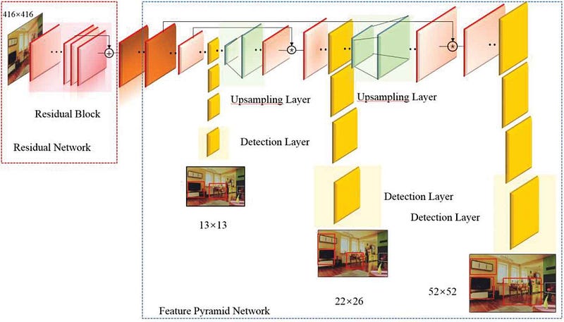
Yolov3 architecture:

1. Input Image

• The input to YOLOv3 is an image (e.g., 416x416 pixels, though the size can vary).
• The image is resized to a fixed dimension to fit the network.

2. Backbone — Darknet-53

• Purpose: Feature extraction from the input image.
• Composed of 53 convolutional layers (hence the name Darknet-53).
• Uses residual connections (similar to ResNet) to improve gradient flow and avoid vanishing gradients.
• Alternates between 3x3 and 1x1 convolutional filters.
• Includes batch normalization and Leaky ReLU activation after each convolution.
• Example: For an input image of size 416×416x3
• Early layers extract low-level features (edges, textures).
• Deeper layers extract high-level features (shapes, objects).

3. What is Feature Pyramid Network (FPN)?

• FPN is a neural network architecture that constructs a pyramid of feature maps at different scales.
• It combines high-resolution, low-level features (fine details) with low-resolution, high-level features (semantic information) to improve object detection across scales.
• In YOLOv3, FPN is used to predict objects at three different scales: 13x13, 26x26, and 52x52

How FPN Works in YOLOv3

YOLOv3 uses a modified version of FPN to generate feature maps at three scales. Here’s how it works:

Predictions at 13x13, 26x26, and 52x52 Grids

After constructing the feature pyramid, YOLOv3 makes predictions at three different scales:

13x13 Grid (Large Objects)

• The 13x13 feature map is derived from the deepest layer of Darknet-53 (Layer 82).
• This feature map has the smallest spatial dimensions but the highest semantic information.
• It is used to detect large objects because the receptive field of each grid cell is large.

26x26 Grid (Medium Objects)

• The 26x26 feature map is derived from an intermediate layer of Darknet-53 (Layer 94).
• This feature map is created by upsampling the 13x13 feature map and concatenating it with a feature map from a shallower layer.
• It is used to detect medium-sized objects.

52x52 Grid (Small Objects)

• The 52x52 feature map is derived from the shallowest layer of Darknet-53 (Layer 106).
• This feature map is created by upsampling the 26x26 feature map and concatenating it with a feature map from an even shallower layer.
• It is used to detect small objects because the receptive field of each grid cell is small.

Note: Upsampling is done using nearest-neighbor interpolation.

4.Anchor Boxes

• YOLOv3 makes predictions at three scales (13x13, 26x26, and 52x52), and each grid cell predicts 3 bounding boxes. Here’s how the total number of detections is calculated:

Predictions per Scale

• 13x13 Scale:
• Grid cells: 13 x 13 = 169.
• Bounding boxes per cell: 3.
• Total predictions: 169 x 3 = 507.
• 26x26 Scale:
• Grid cells: 26 x 26 = 676.
• Bounding boxes per cell: 3.
• Total predictions: 676 x 3 = 2,028.
• 52x52 Scale:
• Grid cells: 52 x 52 = 2,704.
• Bounding boxes per cell: 3.
• Total predictions: 2,704 x 3 = 8,112.

Total Predictions

• The total number of predictions made by YOLOv3 is the sum of predictions at all three scales:
• 507 (13x13) + 2,028 (26x26) + 8,112 (52x52) = 10,647

Note:

Not all 10,647 predictions are final detections. YOLOv3 uses two steps to filter out low-confidence predictions:

Objectness Score Thresholding:

• Predictions with an objectness score below a threshold (e.g., 0.5) are discarded.

Non-Maximum Suppression (NMS):

• Removes overlapping bounding boxes with lower confidence scores, keeping only the most confident predictions.

5.Detection Head in YOLOv3

The detection head consists of a series of convolutional layers applied to the feature maps at three scales (13x13, 26x26, and 52x52). Here’s how it works:

Input to the Detection Head

• The input to the detection head is the feature maps from the FPN at three scales:
• 13x13: For detecting large objects.
• 26x26: For detecting medium-sized objects.
• 52x52: For detecting small objects.

Convolutional Layers

• The detection head applies 1x1 convolutional layers to the feature maps to produce the final predictions.
• Each convolutional layer predicts:
• Bounding box coordinates: 4 values (x, y, width, height).
• Objectness score: 1 value (confidence that the box contains an object).
• Class probabilities: C values (probabilities for each of the C classes).

Output Shape

• For each grid cell in the feature map, the detection head predicts:
• B bounding boxes: YOLOv3 predicts 3 bounding boxes per grid cell (B = 3).
• Each bounding box has 4 coordinates (x, y, width, height),1 objectness score, C class probabilities.
• The output shape of the detection head for a single scale is:(Grid Size x Grid Size) x B x (5 + C)
• For example, for a 13x13 grid with 3 bounding boxes and 80 classes (COCO dataset), the output shape is:13 x 13 x 3 x (5 + 80) = 13 x 13 x 255
• YOLOv3 uses independent logistic classifiers (sigmoid activation) for each class to predict class probabilities.

6.YOLOv3 Loss Function

YOLOv3 introduces several improvements over YOLOv1, including multi-scale detection and a more sophisticated loss function. The loss function in YOLOv3 consists of the following components:

Components of YOLOv3 Loss

Bounding Box Loss (Coordinate Loss):

• Penalizes errors in the predicted bounding box coordinates (x, y, width, height).
• Uses Binary Cross-Entropy (BCE) for the center coordinates (x, y) and MSE for the dimensions (width, height).
• The width and height are predicted as offsets relative to anchor boxes.
• Formula: Loss_coord = λ_coord * Σ [ BCE(tx, tx_gt) + BCE(ty, ty_gt) + MSE(tw, tw_gt) + MSE(th, th_gt) ]

Objectness Loss:

• Penalizes errors in the predicted objectness score (confidence that a bounding box contains an object).
• Uses Binary Cross-Entropy (BCE) for both positive boxes (containing objects) and negative boxes (not containing objects).
• Formula: Loss_obj = Σ [ BCE(C, C_gt) ]

Class Loss:

• Penalizes errors in the predicted class probabilities.
• Uses Binary Cross-Entropy (BCE) for the class probabilities.
• Formula: Loss_class = Σ [ BCE(p(c), p(c)_gt) ]

Total Loss in YOLOv3

The total loss is the sum of the bounding box loss, objectness loss, and class loss:

Total Loss = Loss_coord + Loss_obj + Loss_class

• Pros: Fast, accurate, multi-scale detection, anchor boxes, flexible class prediction.
• Cons: Localization errors, increased complexity, higher computational cost.
• Limitations: Struggles with small objects, overlapping objects, anchor box dependency, data requirements, and hardware needs.