Building a Local Amazon Rufus Clone: Architecture, Hardware Tricks and Hard-Won Lessons

A deep dive into building a full-stack conversational AI shopping assistant — with supply chain intelligence — that runs entirely on your own GPU.

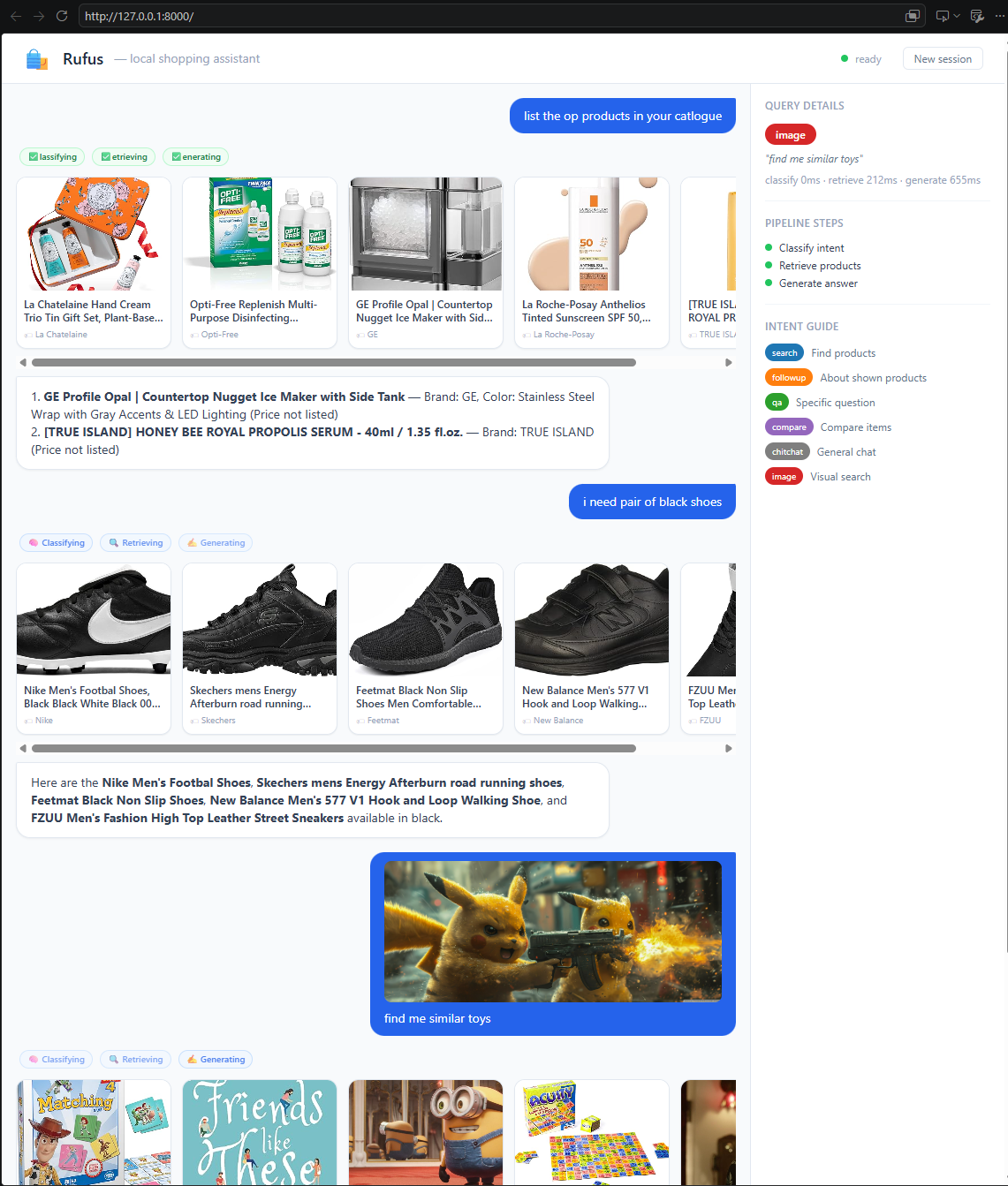
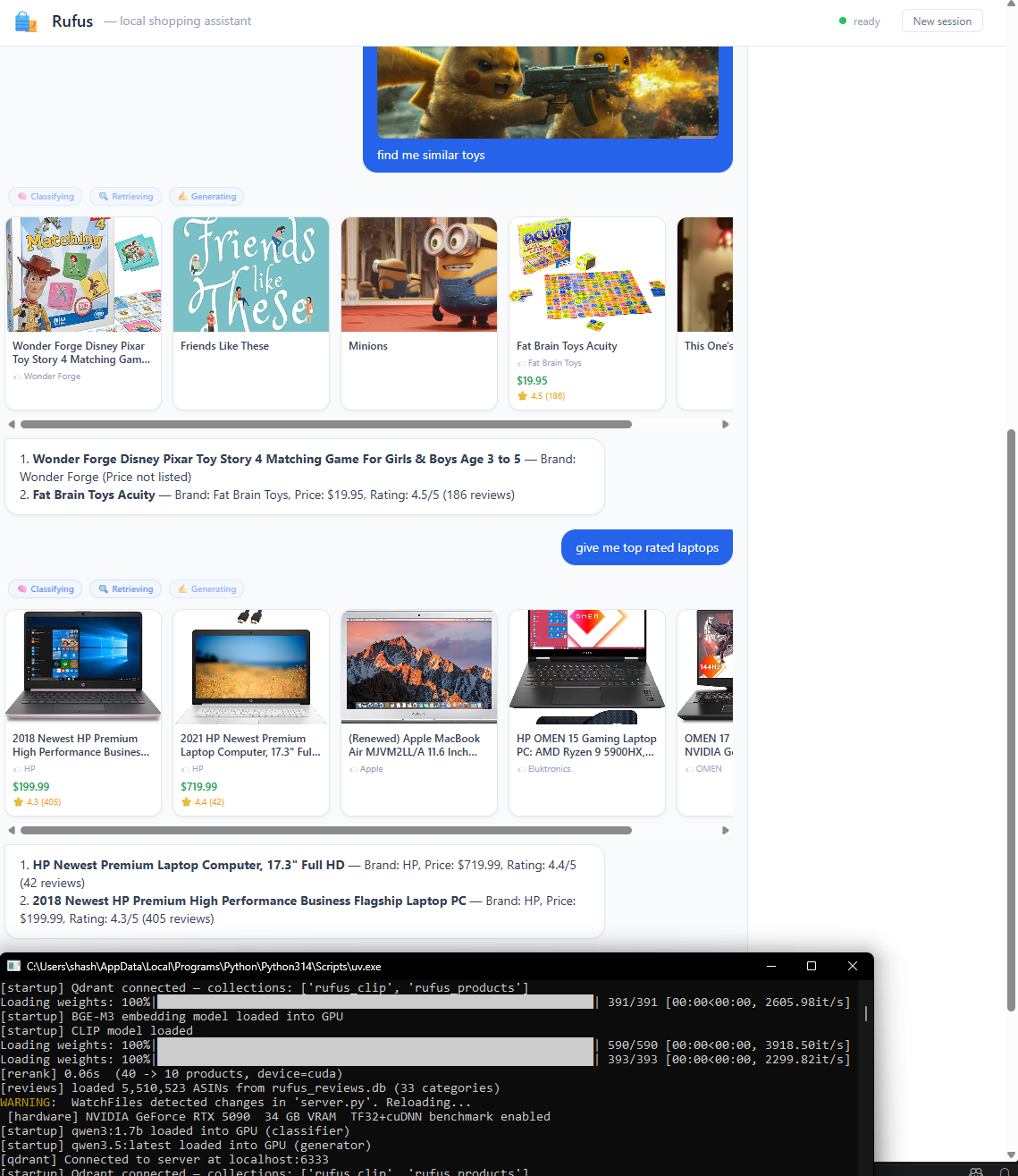
Rufus Lite: a local clone of Amazon’s Rufus AI shopping assistant, running entirely on a single RTX 5090 with no cloud API calls. By the end, the system handles 13 conversation intents, searches 156,000 image-complete products using dual-encoder retrieval, manages a supply chain layer with 110,000 demand forecasts, and streams answers in under four seconds end-to-end.

This post is about the architecture that makes all of that work — the design choices, the hardware tricks, and especially the mistakes that cost me days I’ll never get back.

What We’re Building

The end goal: a user types “show me noise-cancelling headphones under $150” into a chat interface. The system should:

1. Understand what they want (search, not a supply chain query, not a follow-up to a previous result)
2. Find the best matching products across 156K items using both text and image signals
3. Re-rank those results using a cross-encoder for precision
4. Personalize the ranking based on the user’s session history
5. Generate a grounded, non-hallucinating answer that streams back token by token
6. Show actual product images and prices

All in under four seconds, on local hardware.

The Full Pipeline at a Glance

User message (text or image)
        │
        ▼
┌───────────────────────────────────────────────┐
│  CLASSIFY  — fast-path rules (0 ms)           │
│             └─ qwen3.5 LLM fallback (~500 ms) │
└──────────────┬────────────────────────────────┘
               │  intent + clean query + filters
               ▼
   ┌───────────┴──────────────────────────────┐
   │  Shopping intents (search/qa/compare)    │
   │                                          │
   │  RETRIEVE                                │
   │    BGE-M3 (1024-dim fp16) ──┐            │
   │    CLIP ViT-L/14 (768-dim) ─┼─ RRF ─────┤
   │    Personalization signal ──┘            │
   │                   │                      │
   │  RERANK  (bge-reranker-v2-m3, fp16)      │
   │                   │                      │
   │  FILTER  (brand / color / price_max)     │
   └─────────────────┬─────────────────────── ┘
                     │ top-5 products
                     ▼
   ┌─────────────────────────────────────────────┐
   │  GENERATE  — qwen3.5:latest  (streaming)    │
   │  RAG context: title + price + rating +      │
   │              features + review snippet      │
   └────────────────────┬────────────────────────┘
                        │ AG-UI SSE tokens
                        ▼
              Streaming chat UI

   ┌────────────────────────────────────────────┐
   │  Supply chain intents (check_stock, etc.)  │
   │  → SQLite + NeuralForecast → sc_generate   │
   └────────────────────────────────────────────┘

Let’s walk through each layer.

Layer 1 — Intent Classification: Speed Before Correctness

The first thing the system does with every message is figure out what the user actually wants. There are 13 possible intents, from search to reorder_alert. The naive approach — call an LLM for every message — adds 400–800ms of latency before you've even started retrieving products.

The better approach: a two-tier classifier.

Tier 1: Rule-based fast path (0 ms)

_SC_STOCK = (
    "stock level", "qty on hand", "check inventory",
    "inventory level", "show inventory", "check stock",
    "what is out of stock", "out of stock report",
)
def _fast_classify(message: str, has_history: bool) -> dict | None:
    m = message.lower().strip()
    if any(w in m for w in _SC_STOCK):
        return {"intent": "check_stock", "query": message, ...}
    if any(m.startswith(c) for c in _CHITCHAT) and len(m) < 60:
        return {"intent": "chitchat", ...}
    if not has_history and len(_clean_query(message).split()) >= 3:
        return {"intent": "search", "query": _clean_query(message), ...}
    return None  # fall through to LLM

This handles the vast majority of queries: any first-turn message with three or more meaningful words is almost certainly a search. Common chitchat starters, compare words, followup phrases, and supply chain keywords are all caught here in microseconds.

Tier 2: LLM fallback (qwen3.5:latest, ~500 ms)

Only genuinely ambiguous cases — single-word queries like “sarees”, mid-conversation ambiguities, or unusual phrasing — fall through to the LLM:

resp = ollama.chat(
    model="qwen3.5:latest",
    messages=msgs,
    format="json",
    options={"temperature": 0, "num_predict": 128, "num_ctx": 2048},
    keep_alive="60m",
    think=False,
)

The system prompt tells the model to fix typos and expand unusual terms: "saries" → "sarees Indian traditional ethnic dress". Without this, a misspelled one-word query would retrieve nothing useful.

The key insight: you don’t need an LLM for classification in most cases. A well-maintained keyword list and a few simple rules covers 80–90% of traffic at zero latency cost.

Layer 2 — Query Cleaning: What You Send to the Embedder Matters Enormously

Before any query goes into the embedding model, it passes through _clean_query(). This was one of the most impactful and least obvious fixes in the entire project.

The ranking modifier problem

When a user types “best selling sarees,” they want sarees. But the phrase “best selling” appears constantly in Amazon book and music listings — bestseller lists, album charts, chart-toppers. When BGE-M3 encodes “best selling sarees” as a single semantic unit, the embedding drifts toward those book/music neighborhoods in the 1024-dimensional space.

The fix is to strip ranking modifiers before encoding:

_MODIFIER_RE = re.compile(
    r"\b(?:"
    r"best[\s\-]?selling|top[\s\-]?rated|most[\s\-]?popular|"
    r"trending|highly[\s\-]?rated|new[\s\-]?arrivals?|"
    r"affordable|budget[\s\-]?friendly|cheap"
    r")\b\s*",
    re.I,
)
def _clean_query(message: str) -> str:
    cleaned = _MODIFIER_RE.sub(" ", message).strip()
    cleaned = re.sub(r"\s{2,}", " ", cleaned).strip()
    return cleaned if len(cleaned) >= 3 else message

"best selling sarees" → "sarees". The embedding now goes to the right neighborhood.

Note: the modifier stripping applies to the retrieval query only. The original message with all its adjectives is still used for filter extraction (price, color) and is shown to the LLM.

Layer 3 — Dual-Encoder Retrieval: Two Models, One Result

Products in the catalog have two kinds of signal: text (title, bullet points, brand) and images. A pure text retriever misses cases where the user’s intent is visual. A pure image retriever misses semantic nuance. The solution: run both and fuse.

BGE-M3 text retrieval

BGE-M3 from BAAI is one of the strongest open embedding models for retrieval. It encodes the cleaned query into a 1024-dimensional dense vector, then finds the nearest neighbours in Qdrant.

# fp16, batch_size=64 — ~2 ms per query on RTX 5090
self._model = SentenceTransformer(
    "BAAI/bge-m3",
    device="cuda",
    model_kwargs={"torch_dtype": torch.float16}
)
vec = self.model.encode(query, normalize_embeddings=True, batch_size=64)
hits = self._client.query_points(collection_name="rufus_products", ...)

CLIP image-text retrieval

For text queries, CLIP ViT-L/14 encodes the query into the same 768-dimensional space as the pre-computed image embeddings. This allows purely text-described queries to surface products whose image features match the semantic intent.

For image queries (user attaches a photo), the image itself is encoded and searched directly.

# Text query → CLIP space
inputs = self._processor(text=[query], return_tensors="pt", padding=True)
with torch.no_grad(), torch.cuda.amp.autocast():
    text_features = self._model.get_text_features(**inputs)

Reciprocal Rank Fusion

The two retriever outputs are merged using RRF. The formula is simple but powerful:

RRF_K = 60   # dampening constant — reduces the dominance of rank 1

for rank, product in enumerate(results):
    scores[pid] = scores.get(pid, 0.0) + 1.0 / (RRF_K + rank + 1)

A product that appears at rank 1 in both lists gets a far higher fused score than something that appears at rank 1 in only one. Products missing from a list are simply not penalized — they just don’t accumulate that ranker’s contribution.

A subtle bug we hit: after RRF merge, we kept the product object with the highest individual cosine score. BGE-M3 cosine scores (~0.8) always beat CLIP scores (~0.3), so the BGE-M3 product object always “won” — but BGE-M3 objects never carry image_url (it's not stored in BGE-M3's Qdrant collection). The fix: after score-based merge, carry image_url from whichever source has it:

if product.image_url and not best[pid].image_url:
    best[pid] = dataclasses.replace(best[pid], image_url=product.image_url)

Lesson: when merging objects from multiple sources, never assume the winner on one dimension (score) has all the metadata you need.

Layer 4 — Cross-Encoder Reranking: The Precision Layer

Bi-encoders are fast because query and document are encoded independently. But that independence is also their weakness — they can’t model fine-grained interactions between the query and the document.

A cross-encoder sees both at once:

cross-encoder([query, product_title + bullet_points]) → relevance score

We use BAAI/bge-reranker-v2-m3 on the candidate pool (top 40 from RRF), running in fp16 at batch size 128 on the RTX 5090. It re-scores all 40 candidates and returns the best 10, which then get filtered to 5.

scores = self.model.predict(pairs, show_progress_bar=False, batch_size=128)
ranked = sorted(zip(scores, products), key=lambda x: x[0], reverse=True)

On an RTX 5090 this runs in ~30 ms for 40 candidates. The quality improvement is significant — it catches cases where a product has “wireless” deep in its bullet points but not in the title, or where a brand name slightly changes the ranking.

Layer 5 — Personalization: Real-Time Preference Signals

Instead of a static recommendation model, Rufus Lite tracks what the user has actually looked at this session and uses that to bias the retrieval pool.

The mechanism:

1. Every product shown to the user is logged in their session profile (last 20 products)
2. At query time, the BGE-M3 vectors of those viewed products are fetched from Qdrant by payload ID
3. Those vectors are averaged into a “taste centroid”
4. A Qdrant ANN search is run against that centroid to find similar products
5. The results join the RRF pool as a third ranker

def get_similar_to_viewed(session_id: str, top_k: int = 10) -> list[Product]:
    viewed_ids = _get_viewed_ids(session_id)
    if not viewed_ids:
        return []
    # Average the BGE-M3 vectors of all viewed products
    vectors = [get_product_vector(pid) for pid in viewed_ids]
    centroid = [sum(v[i] for v in vectors) / len(vectors) for i in range(1024)]
    return retriever.retrieve_by_vector(centroid, top_k=top_k)

For new sessions with no history, deterministic seed profiles (5 user archetypes) provide a prior based on a hash of the session ID. This avoids the cold-start void where new users get identical, unbiased results.

Layer 6 — RAG Context and Generation: The Hardest Part to Get Right

Retrieval is a solved problem compared to generation. Getting the LLM to stay grounded in the actual data — never inventing prices, not hallucinating specs, not copying internal metadata into the answer — took more iteration than the entire retrieval stack.

Context formatting

Each product in the RAG context is formatted as a single structured line:

1. **Sony WH-1000XM5 Wireless Headphones** — Brand: Sony, Color: Black,
   Price: $279.99, Rating: 4.8/5 (12,847 reviews)
   Features: Industry-leading noise cancelling • 30-hour battery
   Review: "The best noise cancellation I've ever experienced..."

The SYSTEM_PROMPT

Anti-hallucination rules must be stated with zero ambiguity. Soft guidance (“try to avoid inventing prices”) doesn’t work:

RULES — follow every time, no exceptions:
1. Use ONLY the product data provided. Never invent specs, prices, ratings.
2. PRICE: If a product has "Price: not listed", do NOT mention a price — omit it entirely.
3. RATINGS: Only mention ratings if they are explicitly shown in the product data.
4. Always format product names in **bold**.
5. Keep answers under 120 words.
6. Do not start with "I" or "Sure" or "Of course".
7. NEVER guess or estimate any data not explicitly provided.

Point 2 is the critical one. Without the explicit “omit it entirely,” a model that knows the product category will reason: “electronics in this range typically cost $X” and produce that number. You want the model to find “Price: not listed” and stop thinking about price entirely.

Model choice: qwen3.5:latest over qwen3:1.7b

The initial system used qwen3:1.7b for both classification and generation. It was fast (~300ms TTFT) but consistently hallucinated prices and had no knowledge of non-English product categories. When a user typed "kurta" (Indian men's traditional clothing), the 1.7b model had no idea and returned generic shirts.

Switching generation to qwen3.5:latest (6.6 GB, Q4 quantization) eliminated hallucinated prices entirely and correctly handled domain-specific terms. The speed trade-off is real — TTFT increases to ~2.5s — but answer quality is dramatically better.

Layer 7 — Supply Chain: When the Same LLM Needs to Wear a Different Hat

Beyond shopping, the system handles five supply chain intents:

Intent What it does check_stock "Is the Anker USB-C charger in stock?" → SQLite inventory lookup reorder_alert "What needs to be reordered?" → urgency-scored alert list demand_forecast "Forecast demand for headphones" → NeuralForecast NHITS 30-day supplier_query "Who are our suppliers?" → supplier table with lead times sc_analytics "Show inventory health" → category summary + critical items

The routing happens in the same classifier as shopping intents but uses a separate system prompt with completely different rules. The SC prompt is even stricter about data fidelity:

1. Report ONLY data explicitly provided. Never invent SKU names, supplier names, quantities.
2. If a SKU looks like a hash code (e.g. "9dc1a7de"), report it verbatim.
3. If the data section says "No inventory data found", say so — do NOT invent placeholder data.

The forecasts themselves are generated by NeuralForecast NHITS, a neural sequence model that runs on GPU. On the RTX 5090, training 3,693 inventory SKUs across 30 days takes approximately six seconds. The key configuration detail: start_padding_enabled=True, which lets the model train on time series shorter than input_size — without it, any SKU with fewer than 30 historical data points is silently skipped.

Hardware: Making an RTX 5090 Actually Work

fp16 everywhere

Every inference model runs in fp16:

# BGE-M3
SentenceTransformer("BAAI/bge-m3", model_kwargs={"torch_dtype": torch.float16})
# CLIP
CLIPModel.from_pretrained("openai/clip-vit-large-patch14",
                          torch_dtype=torch.float16)
# Cross-encoder reranker
CrossEncoder("BAAI/bge-reranker-v2-m3",
             model_kwargs={"torch_dtype": torch.float16})

fp16 roughly halves memory bandwidth requirements and doubles throughput on tensor cores compared to fp32. On a 32 GB card, the savings let you keep multiple models in VRAM simultaneously.

TF32 and cuDNN benchmark

Applied once at import time via rufus/hardware.py:

torch.set_float32_matmul_precision("high")   # TF32 on matmul ops
torch.backends.cuda.matmul.allow_tf32 = True
torch.backends.cudnn.allow_tf32 = True
torch.backends.cudnn.benchmark = True         # auto-selects fastest kernels

cudnn.benchmark = True is worth understanding: on first run, cuDNN profiles several convolution kernel implementations and caches the fastest one for each input shape. If your input shapes are fixed (which they are for embedding — every query encodes a text string of similar length), the speedup compounds over thousands of calls.

Keep Ollama models pinned in VRAM

Ollama unloads models from VRAM after a period of inactivity. For a latency-sensitive API, you cannot afford a 15-second model reload on the first request after a quiet period.

ollama.chat(model="qwen3.5:latest",
            messages=warmup_msgs,
            options={"num_predict": 1},
            keep_alive="60m")  # stays loaded for 60 minutes

Run this at server startup for every model the app uses. Combined with keep_alive on every subsequent call, the model stays in VRAM indefinitely.

Startup warmup: eliminate cold-start on first request

Without warmup, the first request after a server restart pays the cost of loading every model from disk. For BGE-M3, that’s 15–20 seconds. For the cross-encoder reranker, the first inference also triggers CUDA kernel compilation — another 30–60 seconds.

The fix: a startup hook that loads everything before the server begins serving:

@app.on_event("startup")
async def _warmup():
    loop = asyncio.get_event_loop()
    async def _load():
        # 1. LLM models — pin in Ollama VRAM
        ollama.chat(model="qwen3:1.7b", ..., keep_alive="60m")
        ollama.chat(model="qwen3.5:latest", ..., keep_alive="60m", think=False)
        # 2. Qdrant connection - ensures server mode before first query
        get_client().get_collections()
        # 3. BGE-M3 - eliminates 18s cold-start on first search
        _get_retriever()   # creates ProductRetriever and loads model to GPU
        # 4. CLIP
        _get_clip()
    await loop.run_in_executor(None, _load)

After warmup: retrieve ~300ms, generate ~2s, total under 4s.

LLM context window is a performance dial, not just a memory limit

num_ctx in Ollama controls the KV cache size. Larger values allow longer context but increase per-token computation — the attention mechanism is O(context²).

For Rufus Lite’s use case, the full prompt is rarely more than ~700 tokens (system prompt + 5 products + user question). Setting num_ctx=2048 instead of 4096 roughly halves first-token latency on qwen3.5:latest while safely covering all real inputs.

opts = {"num_ctx": 2048, "num_predict": 256, "temperature": 0}

num_predict=256 caps the maximum generation length. A shopping assistant answer should never exceed 120 words — if the model hits 256 tokens, it was rambling.

The Qdrant Production Lesson: Startup Order Is a Contract

Qdrant offers two modes:

• Server mode (localhost:6333) — runs as a separate process, manages memory via OS mmap, supports concurrent access
• Local file mode (QdrantClient(path="...")) — opens the storage directory directly in the Python process

Local file mode seems convenient for development. But it has a fatal flaw in production: it acquires an exclusive file lock on the storage directory. If two processes try to open it simultaneously, the second one fails. More subtly: if you start your Python server before the Qdrant binary is running, it falls back to local file mode. When you then start the Qdrant binary, it takes the exclusive lock — and every subsequent query from your Python process fails with Collection rufus_products not found.

The fix has two parts:

1. Always start Qdrant before the application server.

2. Make the singleton auto-reconnect:

_client_mode: str = "none"   # "server" | "local" | "none"
def get_client() -> QdrantClient:
    global _client, _client_mode
    if _client is not None:
        # If we're in local-file mode, try upgrading to server
        if _client_mode == "local":
            server = _try_server()
            if server is not None:
                _client.close()
                _client = server
                _client_mode = "server"
        return _client

With this logic, if the startup ordering was wrong, the first request that actually reaches the retriever will trigger a reconnect to the now-running server. The user sees one failed request instead of every request failing forever.

Caching: The 80/20 Rule Applied to Retrieval

Shopping queries are highly repetitive. “Wireless headphones,” “running shoes,” “coffee maker” — a small number of queries account for most traffic. Two cache layers exploit this:

# Embedding vectors — deterministic per model, never expire
embedding_cache = LRUCache(maxsize=2048, ttl=None)
# Rerank results - expire after 5 minutes (catalog can change)
rerank_cache = LRUCache(maxsize=512, ttl=5 * 60)

The embedding cache is particularly effective: BGE-M3 encoding takes ~2ms, but for a repeated query it’s 0ms. The LRU with 2048 entries holds all “typical” shopping queries comfortably — at 1024 floats per vector (fp32 in cache) that’s 8 MB total.

Thread safety matters: these caches are shared across all request-handling threads. Every operation acquires a lock.

The AG-UI Protocol: Streaming Without Polling

The frontend communicates with the server via Server-Sent Events following the AG-UI protocol. Every step in the pipeline emits structured events:

RunStarted
  StepStarted("classify")
    CustomEvent("intent", {intent, query, filters})
  StepFinished("classify")
  StepStarted("retrieve")
    CustomEvent("products", [...])
  StepFinished("retrieve")
  StepStarted("generate")
    TextMessageStart
    TextMessageContent × N   ← each LLM token
    TextMessageEnd
  StepFinished("generate")
RunFinished

The UI renders the step chip (“🔍 Retrieving…”) immediately on StepStarted, shows product cards on the CustomEvent("products"), and streams tokens in real time as TextMessageContent events arrive.

The pipeline runs in a background thread while an async queue feeds the SSE stream:

@app.post("/awp")
async def agent_endpoint(body: RunAgentInput):
    queue = asyncio.Queue()
    loop = asyncio.get_event_loop()
    thread = threading.Thread(
        target=_run_pipeline, args=(body, queue, loop), daemon=True
    )
    thread.start()
async def event_stream():
        while True:
            chunk = await queue.get()
            if chunk is None:
                break
            yield chunk
    return StreamingResponse(event_stream(), media_type="text/event-stream")

This pattern lets the blocking LLM call run in a thread without blocking the event loop, while the async generator pushes each token to the client as soon as it’s emitted.

Production Reliability: The Non-Glamorous Work

Circuit breaker for Ollama

Ollama is a separate process. It can crash, hang, or become unresponsive. Without protection, a hung Ollama call blocks a request thread forever — eventually exhausting the thread pool.

class _CircuitBreaker:
    # Closed → (3 failures) → Open → (60s) → Half-Open → (success) → Closed
    def allow(self) -> bool: ...
    def record_success(self) -> None: ...
    def record_failure(self) -> None: ...

When the breaker is open, OllamaClient.chat() returns None immediately. The server then shows the retrieved products without a generated answer — degraded but functional.

Retry with exponential backoff

Transient failures (network hiccup, model briefly busy) are retried with jitter:

for attempt in range(MAX_RETRIES + 1):
    if attempt > 0:
        sleep = BASE_BACKOFF * (2 ** (attempt - 1)) + random.uniform(0, 0.3)
        time.sleep(sleep)
    try:
        return ollama.chat(...)
    except Exception:
        pass

Jitter (+ random.uniform(0, 0.3)) prevents the thundering herd: if five requests all fail simultaneously and retry at the same interval, they all hit Ollama again at the same moment.

Dos and Don’ts: The Lessons That Cost the Most Time

DO: Strip ranking modifiers before embedding. “Best selling sarees” encodes differently from “sarees.” The modifier pulls the vector toward Amazon bestseller books. Strip it before encoding; use it only for metadata (the user did say “best selling,” which could inform display ordering).

DON’T: Pass think=False inside Ollama's options dict.

# WRONG — routes all output to the .thinking field, content is empty
ollama.chat(model="qwen3", options={"think": False, ...})
# RIGHT - think=False as a direct kwarg
ollama.chat(model="qwen3", options={...}, think=False)

This cost an entire afternoon. The model appeared to return successfully but with zero content — message.content was empty because all tokens went to message.thinking. No error, no warning.

DO: Use Qdrant in server mode, never local-file mode at scale. Local file mode above 20K vectors is slow (every query reads from SQLite) and exclusively locks the storage directory. The standalone Qdrant binary takes two minutes to set up and eliminates both problems.

DON’T: Use Python’s or operator to handle DataFrame returns.

# WRONG — raises "The truth value of a DataFrame is ambiguous"
pred = _gpu_forecast() or _rolling_fallback()
# RIGHT - always use explicit None check
pred = _gpu_forecast()
if pred is None:
    pred = _rolling_fallback()

This will bite you in any ML pipeline that returns DataFrames. Always.

DO: Remove internal metadata from LLM context. If you put (relevance: 0.99) in the context you send to the LLM, the LLM will copy it into the answer. Users should not see retrieval scores, internal field names, debug flags, or system identifiers.

DON’T: Assume “omit” means “don’t mention” for price. Saying “omit price if not listed” in the system prompt isn’t enough. The model knows what category of product it’s looking at and will reason about a typical price. Be explicit: “If a product has ‘Price: not listed’, do NOT mention a price for it — omit it entirely.”

DO: Pre-warm every model at server startup. Every model you lazy-load will cause a latency spike on the first request that needs it. BGE-M3 takes 15–20 seconds to load from disk to GPU. The cross-encoder reranker needs CUDA kernel compilation on first inference (~60s). Wire up a startup hook that loads everything before the server begins accepting traffic.

DON’T: Assume your LangGraph pipeline and your FastAPI server use the same code path. If you build a LangGraph graph for the conversation pipeline and also a FastAPI server that handles production traffic, any node you add to the graph is NOT automatically in the server’s pipeline. Every significant change must be applied to both. This sounds obvious until 3am when you’re debugging why supply chain intents work in the REPL but not the UI.

DO: Use SHA-256 for stable product IDs. Python’s built-in hash() is not stable across process restarts (it's randomized by default for security). If you use it to generate Qdrant point IDs during ingestion, every server restart produces different IDs — and your product catalog becomes unsearchable.

# WRONG
product_id = hash(f"{source}:{title}")
# RIGHT
product_id = hashlib.sha256(f"{source}:{title}".encode()).hexdigest()[:16]

DO: Keep num_ctx as small as safely possible. The attention mechanism is quadratic in context length. For a shopping assistant that generates short answers from a compact RAG context, num_ctx=2048 is sufficient and meaningfully faster than 4096. Measure your actual prompt lengths before setting this.

DON’T: Train time-series models and use their raw output dates. A forecasting model trained on data from 2016 will generate predictions dated 2016. Any query filtering on forecast_date >= today will return zero results. Always remap model output dates to today + offset before storing:

for i, (_, row) in enumerate(sorted_predictions):
    row["forecast_date"] = (today + timedelta(days=i)).isoformat()

Performance Summary

Component Cold Warm Fast-path classify 0 ms 0 ms LLM classify (qwen3.5) ~15s (load) ~500 ms BGE-M3 encode ~18s (load) ~2 ms Qdrant ANN search ~5 ms ~5 ms CLIP encode ~10s (load) ~4 ms RRF fusion <1 ms <1 ms Cross-encoder rerank (40→5) ~60s (compile) ~30 ms qwen3.5 generate (TTFT) ~20s (load) ~2.5s End-to-end ~60–90s ~3–4s

The startup warmup hook eliminates the “Cold” column for production traffic. After warmup completes (~30s after server start), every request lands in the “Warm” row.

What I’d Do Differently

Start Qdrant in Docker from day one. The standalone binary works, but Docker Compose (docker compose up -d qdrant) gives you restart policies, health checks, and volume management for free. The local file mode fallback sounds convenient and caused a multi-hour debugging session.

Use a smaller catalog and add products incrementally. Starting with 156K image-complete products was a late decision (after rebuilding from 1.2M). The smaller, higher-quality catalog gives better results than a massive catalog where 90% of products have no image and sparse metadata.

Measure before optimizing LLM calls. I assumed qwen3:1.7b was fast enough and qwen3.5:latest was too slow. When I actually measured: warm generation for a 100-word answer took ~800ms with qwen3.5:latest. The quality difference was enormous, the speed difference was acceptable.

Add the circuit breaker first, not last. It took a hung Ollama process taking down the entire request thread pool to motivate adding the circuit breaker. It should be the first reliability layer added to any LLM-dependent service.

Closing Thoughts

Building a full-stack conversational AI system on local hardware is entirely feasible today — but the interesting engineering is not in the ML models. The models are readily available and well-documented. The interesting work is in the integration layer: how you clean queries before they reach the embedder, how you merge signals from multiple retrieval systems, how you prevent the LLM from hallucinating into your grounded context, and how you make all of it survive the operational realities of startup ordering, cold starts, and process failures.

The RTX 5090 with 32 GB VRAM makes running multiple large models simultaneously practical. fp16 inference, TF32 matmul, and cuDNN’s auto-tuner mean most of the hardware is being used efficiently. The models themselves are now fast enough that the bottleneck has shifted back to the application layer — which is exactly where it should be.

The full source code for Rufus Lite is available at github.com/shashanka300/rufus_lite.