Enhancing time series foundation models at Decathlon: from covariates to robust ensembling

In our previous article, **The TSFM Showdown: Who’s Winning the Forecasting Battle at Decathlon?, we assessed the raw potential of Time Series Foundation Models (TSFMs) on purely historical data. Now, we answer the next critical question: how do we push them further?**

A primary challenge in retail demand forecasting lies in the effective integration of covariates. External factors are essential for explaining sales volatility. With the emergence of TSFMs, leveraging these covariates has become a key area of exploration. However, feature engineering is only half the battle; the other half is synergy. By combining predictions from multiple models, we can achieve results where ‘the whole is greater than the sum of its parts’. This article explores these two pillars: covariate integration and model ensembling within the context of our specialized retail datasets.

Breaking the Glass Ceiling: Native Covariate Integration with Chronos-2

Covariates specification

Different covariates were tested as prices, stores count and weather.

Price: This represents the weekly base price of a product. While this price is dynamic and can change over time, it excludes promotional discounts.

Weather: We utilize three time series: weekly average temperature, rainfall, and snowfall. Since our forecasting method operates at a European scale, these metrics are calculated as a weighted average across our European stores. For future time steps (the forecasting horizon), we feed the model the average of the past three years of weather data to provide a global seasonal trend.

Store Features: We incorporate two key time series.

• Store count: For each product and week, we calculate the percentage of stores selling the item. Since store assortments are planned ahead, this feature is known in advance.
• Product Range: This is an integer value (1 to 5) representing a product’s level of specialization and technicality. It can change over time

Models tested

Almost every foundation model relies solely on historical time series and cannot handle covariates natively. The standard workaround was often to use a regressor on the residuals. For instance, TimesFM proposed a linear regression on the error, while Chronos-Bolt offered a choice between XGBoost, CatBoost, or LightGBM to regress on the residuals. We tested these options, but no improvements were observed compared to the standalone model.

The real breakthrough came with the release of Chronos-2 by Amazon. As detailed in our previous article, this was already the top-performing foundation model on our data. With its novel architecture , it allows the use of information from different time series like covariates to compute the forecast of a target series. The results presented below are based on this model.

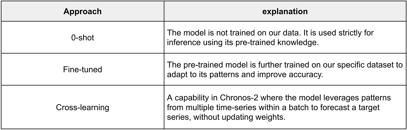
Chronos-2 offers a wide range of options to achieve optimal results. To better understand the performance benchmarks that follow, let’s quickly review the different approaches :

Results for global covariates

We evaluated the impact of store features, price and weather across the entire European catalog (25,000 products). To ensure statistical robustness, we tested these covariates over 52 rolling cutoffs spanning a full year.

Data and scope:

• Time Series: weekly sales frequency, often exhibiting strong seasonal patterns.
• Covariates : Price, weather and stores features.
• History: an average of 4 years of historical data for each product (shorter time series have to be extended synthetically).
• Cutoffs: we benchmarked the models over 52 cutoffs spanning one entire year, from week 37 of 2023 (2023–37) to week 37 of 2024 (2024–37). For each cutoff, we predict and evaluate the performance of the models.
• Scale: Approximately 25,000 unique products to forecast per cutoff with perimeter variation (end of life, new products).

Metrics (ordered by business impact):

• **WAPE **(Weighted Absolute Percentage Error) up to 12 weeks: our most critical metric, corresponding to the replenishment horizon. This metric is reviewed weekly with purchase planners.
• WAPE up to 52 weeks: the long-term horizon, important for strategic stock projection.
• Secondary Metrics: RMSE (Root Mean Squared Error) were used for comparative analysis but are not monitored in production.

Leaderboard:

To evaluate the impact of external features, we compared our fine-tuned Chronos-2 Baseline against three variants: one enriched with Price, one with Store Features and one enriched with weather covariates. We tracked performance across short-term (12 weeks) and long-term (52 weeks) horizons.

Fine-tuning: The benchmark comprises 52 cutoffs spanning a full year, during which fine-tuning is conducted twice. Each fine-tuned model remains in use until the subsequent fine-tuning operation occurs.

Main metrics at both horizon 12 weeks and 52 weeks

At a 12-week horizon, the performance across all variants is almost identical, indicating that these covariates offer limited marginal gains in the short term against a strong baseline. However, at the 52-week horizon, the Store Features variant demonstrates superior accuracy, delivering the lowest WAPE and RMSE.

The minimal impact of the price covariate is likely data-driven: since our current dataset captures standard pricing rather than promotional dynamics, the signal is insufficient to influence the forecast. Similarly, the weather features failed to improve global metrics. This called for more experiments. Even though a large part of our catalogue is expected to be insensitive to weather conditions, others strongly depend on it. As a result, provided no overfitting occurs, we should at least observe some minor improvements. To truly assess the value of weather data, we will isolate and analyze specific weather-dependent product categories.

A Weather Expert Built on a Foundation Model

At Decathlon, a specific subset of our products is highly sensitive to weather conditions. Sales for these items are volatile; for instance, sales of gloves spike significantly during cold spells. We have identified a cluster named winterpeak of approximately 2,000 of these weather-dependent products which represents around 8% of the catalog.

Correlation: Glove Sales and Temperature

On this cluster, we compared different versions of Chronos-2 with weather covariate. It is interesting to note that the zero-shot version, utilizing weather covariates and cross-learning within the cluster, emerged as the best performing ‘local expert’ doing better than the fine-tuned version with weather covariates for instance.

Metrics on the winterpeak cluster from 2023–37 to 2024–37 with products with more than 2 years of sales

The Results:

• Short-Term Win: This “local expert” improved WAPE 12 by ~1 point (26.6% vs 27.7%) compared to the global baseline.
• The Trade-off: While excellent for replenishment, this specialization degraded performance on the long-term horizon (52 weeks).
• Understanding : As demonstrated, the results are more accurate when the model is given ‘perfect’ future weather. This confirms that weather is a key driver of sales and that the model effectively captures this signal. It also highlights that our final forecasting accuracy is heavily dependent on the quality of the weather forecasts.

The following qualitative analysis and visualizations are based on the best-performing configurationat short horizon : Chronos-2 (0-shot) with weather covariates and cross-learning among the Winter Peak cluster.

Visual Proof: As shown in the neck warmer example below, the baseline treats sudden spikes as noise. In contrast, the weather-aware model more accurately links the temperature drop to the sales surge. The temperature given (red curve) is the average of the past 3-years.

Forecasting response to synthetic temperature variations

Does the model really understand weather impact ?

To prove the model captures the weather impact, we perform a sensitivity analysis by artificially lowering the input temperature given in the future (as seen in the red line below). By comparing this test against the baseline, we isolate the specific impact of weather. The sharp rise in predicted sales (the blue peak) confirms the algorithm has correctly learned that temperature drops are a causal signal for demand, validating its alignment with physical reality.

Forecasting response to synthetic temperature variations

Limitations and business use case

• The algorithm’s reliance on accurate weather forecasts introduces a degree of instability when evaluated strictly on forecast accuracy. Large discrepancies between predicted and actual weather conditions directly degrade sales predictions. Specifically, while the results presented above for the winter of 2023–2024 were robust, performance declined during the winter of 2024–2025 because the accuracy of the weather given in the future was poorer.
• However, from a replenishment perspective, this sensitivity transforms into a strategic asset. The model’s capacity to capture weather impact could allow us to simulate different weather scenarios for the upcoming season (e.g., a “mild winter” vs. a “harsh winter”). This could empowers supply chain teams to anticipate demand ranges rather than a single fixed number, enabling better risk management by securing stock for potential cold snaps while avoiding overstocking if conditions remain mild.

Combining forecasts

Combining forecasts is a well-established way to improve accuracy and our results confirm this once again. As shown in our previous article, although Chronos-2 significantly outperforms other foundation models on our benchmark, the pairwise win-rate analysis reveals an important nuance: so-called weaker models still outperform Chronos-2 on roughly 40% of Decathlon products. This diversity of strengths naturally calls for ensembling.

While many ensemble strategies have been proposed in the literature, there is still limited empirical guidance on which approaches work best at scale. At Decathlon, we currently rely on an Online Expert agregation framework to combine forecasts, a dynamic approach we loosely refer to as Mixture of Experts (MoE). This approach produces a convex combination of expert predictions, with weights updated weekly based on the performance with a Bernstein Online Algorithm (BOA).

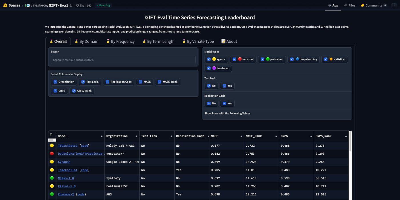
However, it is worth noting that on the GIFT-Eval benchmark, simple ensembling strategies such as the median ensemble proposed by TimeCopilot also achieved strong performance, raising the question of whether this holds true for our datasets.

From Local to Global: Weight Granularity Matters

A key design choice in the MoE systems is how weights are shared across products. Rather than having one weight per time series, we explore several levels of aggregation using our product hierarchy.

The following granularities are evaluated on our global dataset of 25,000 weekly time series:

• Model: one weight per individual time series.
• Family: ~22 time series per group.
• Department: ~450 time series per group.
• Universe: ~1,500 time series per group.
• Global: a single weight for the entire dataset.

Benchmark Setup

This benchmark differs slightly from our previous experiments on covariates. We evaluate forecasts using rolling cutoffs over a one-year period, from week 2023–44 to 2024–44. We consider two expert pools:

• 5 experts: Chronos-2 (fine-tuned), Chronos-Bolt Base (fine-tuned), TimesFM 2.0 (zero-shot), TiRex (zero-shot), Moirai-2 (zero-shot).
• Top 3 experts: Chronos-2 (fine-tuned), Chronos-Bolt Base (fine-tuned), TimesFM 2.0 (zero-shot).

Leaderboard

Main metrics at horizon 12

Main metrics at horizon 52

As expected, combining multiple forecasts outperforms the single best expert. Interestingly, we found that aggregating weights at a coarser granularity (higher levels of the hierarchy) significantly enhances MoE performance, likely by mitigating the overfitting risks associated with item-level noise. Simple ensembling techniques, such as mean or median ensemble, continue to yield strong results.

The Forecast Combination Puzzle: A Two-Model Case Study at Decathlon

We will take a deep dive into the performance of different ensembling strategies. Specifically, we aim to combine two strong but complementary models that have similar performances on our dataset.

• Temporal Fusion Transformer (TFT) — our current production model.
• Chronos-2 (fine-tuned) — the foundation model with the best standalone performance on our benchmark.

Please note that the results for Chronos-2 presented here may differ slightly from earlier sections due to differences in the input data scope.

Main metrics at horizon 12

Main metrics at horizon 52

A Surprising Result

As the metrics shows, simply taking the average ensemble shows strong performance and outperforms Mixture of Experts strategy in this case. This result is not a bug. It is a well-known paradox.

What is the “Forecast Combination Puzzle”?

This phenomenon was identified by Smith and Wallis in 2009. It describes a situation where simple, fixed-weight combinations (like a 50/50 split) sometimes beat more sophisticated methods where weights are estimated from data.

Let us compare:

• a static strategy with a fixed weight *w** ,
• a dynamic strategy with a time-varying weight W.

We define:

The Mean Squared Error (MSE) of the dynamic forecast decomposes as:

Definition of Variables :

Dynamic Adjustment : The “risk-taking” relative to the fixed weight (equals zero if *W is constant and equal to w**).

Static Error : The error the model would have made with a fixed weight strategy.

Interpretation

• Term 2 (Cost of instability) : This term is always positive. Varying weights mechanically introduces variance, which naturally increases the total error.
• Term 3 (Adaptative Gain) : This is the term capable of reducing the total error. To outperform a static strategy, there must be a strong positive covariance between the static error and the dynamic adjustment (meaning the adjustment correctly offsets the error).
• Term 4 (Biais Shift) : This term is negligible, as you can see in the above benchmark the bias variation between the different strategy are small compared to the variation of MSE.

The logic follows a fundamental trade-off:

For a dynamic weight strategy to beat a fixed weight, the reduction in error gained by moving the weight must be greater than the variance of the error introduced by calculating that weight. In some real-world scenarios, especially when 2 algorithms seem to have similar performances, the “cost” of moving the weights is higher than the benefit, making the simple average or median a robust choice.

From theory to practice

The graph above illustrates the WAPE 52 performance comparison between two distinct strategies across our benchmark. The blue curve represents the error at horizon 52 achieved by using various constant fixed weights *w**, while the red point depicts the performance of the Mixture of Experts (MoE) using one weight for the entire dataset. The abscissa of the red point indicates the average weight the MoE assigned to Chronos-2 over the evaluation period.

We observe a classic manifestation of the Forecast Combination Puzzle: although the MoE’s average weight is positioned near the minimum of the blue curve, its actual performance sits above the curve. This vertical gap represents the cost of instability.

While the exact optimal fixed weight cannot be known in advance, a simple equal-weighted approach w* = 0.5 would have yielded superior results to the dynamic MoE in this scenario. This suggests that the “intelligence gain” from dynamic weighting was insufficient to offset the variance introduced by the shifting weights in this example.

As shown in the graph below, the BOA algorithm computes oscillating weights, with no clear winner emerging between the two experts. These fluctuations likely stem from forecast instability across cutoffs, driven by the experts’ sensitivity to the last observed sales point.

Evolution of the weights assigned to each expert by the MoE

While MoE successfully beats the best expert and can capture local behavior which static weights naturally ignore, it remains a fascinating result that the humble stability of a simple median or average can rival such sophistication when looking solely at global accuracy.

Conclusion

Time Series Foundation Models have proven to be highly effective, delivering impressive results with remarkably low development effort. Our benchmarks show that with simple fine-tuning, these models already rival the state-of-the-art algorithms currently in production. However, raw performance was only the first step. To unlock their full potential, the path forward clearly lies in enriching these models with external covariates and leveraging model ensembling.

Key points :

• Foundation models: from global giants to local weather experts Time Series Foundation Models like Chronos-2 are global algorithms designed to generalize across vast datasets, so one would not intuitively expect them to excel as specialized “local experts”. However, the results show a surprising versatility: by utilizing native covariates and cross-learning, it creates a powerful complementary tool: a Foundation Model capable of acting as a “sniper” for weather-sensitive replenishment decisions.
• Combining models always yields gains Ensembling forecasts is a proven method for improving accuracy and consistently outperforms relying on a single “best” expert. This is largely because different models have different strengths; even models considered “weaker” overall were found to outperform the top model on approximately 40% of the products, making their inclusion in an ensemble valuable. Our Mixture of Experts strategy delivered significant performance boosts by leveraging multiple foundation models.
• Simple methods are often surprisingly robust While dynamic weighting systems (like Mixture of Experts) offer significant theoretical advantages, simple ensembling techniques often remain a strong baseline. This is particularly true in specific use cases, where the underlying experts exhibit very similar performance levels. This is related to the ‘Forecast Combination Puzzle,’ where the added complexity of estimating dynamic weights can sometimes offset their benefits, making simple, fixed-weight strategies a computationally efficient and reliable alternative in this specific use-case.