Rebuilding Maps from Pixels: The Power of Image-Driven Reconstruction

Introduction

Maps are one of humanity’s oldest tools for understanding the world. But what happens when those maps are incomplete, flattened, or missing the metadata needed for traditional reconstruction?

In many real-world scenarios — disaster zones, old survey archives, hand-drawn blueprints, low-resolution images — there is little to no structured data available. Yet, modern applications demand 3D context, accurate boundaries, terrain elevation, and more.

The good news? Image processing + intelligent inference can rebuild maps even when data is minimal. Welcome to a world where no data is not a deal-breaker anymore.

The Core Concept: From Pixels to Vectors

The goal is to reverse-engineer a structured dataset from a flat image. This process is often called raster-to-vector conversion or map digitization.

Input: A map image (e.g., a PNG, JPG screenshot of a web map, a scanned paper map, or a chart). Output: Geospatial data (e.g., GeoJSON, Shapefile, KML) or structured data (e.g., CSV with coordinates) that you can analyze in tools like QGIS, ArcGIS, Python (with GeoPandas), or a database.

The Image Processing Pipeline: A Step-by-Step Guide

Let’s walk through the general workflow. We’ll use the example of extracting country boundaries from a simple world map image.

Step 1: Preprocessing — Cleaning the Image

The raw image is often messy. We need to clean it up to make the features we care about stand out.

• Color Thresholding / Segmentation: Isolate the features of interest by their color.
• Example: If the land masses are green and the ocean is blue, we can create a mask where every pixel that is “green” becomes white (1) and everything else becomes black (0).
• Tools: cv2.inRange() in OpenCV (Python) is perfect for this.
• Grayscale Conversion & Binarization: If the map is already monochrome, convert it to a simple black-and-white (binary) image.
• Tools: cv2.cvtColor() and cv2.threshold().
• Noise Removal: Remove small specks of noise (salt-and-pepper) that can confuse the extraction process.
• Tools: Morphological operations like erosion and dilation (cv2.erode(), cv2.dilate()) or filters like median blur (cv2.medianBlur()).

Before Preprocessing: A colorful, noisy map image. After Preprocessing: A clean, binary image where the features are stark white shapes on a black background.

Step 2: Feature Extraction — Finding the Shapes

Now we identify the individual shapes (contours) in our cleaned image.

• Contour Detection: This algorithm finds the boundaries of the white shapes.
• Tools: cv2.findContours() in OpenCV. It returns a list of contours, where each contour is a list of (x, y) coordinates that form the boundary of the shape.
• Approximation: The raw contours might have thousands of points. We can often simplify them without losing significant shape information.
• Tools: cv2.approxPolyDP() uses the Ramer-Douglas-Peucker algorithm to reduce the number of points in a curve.

Result: We now have a mathematical representation of each country’s boundary as a series of points.

Step 3: Georeferencing — From Pixel Space to Real-World Coordinates

This is the “Unflattening” magic. A pixel coordinate (e.g., [150, 300]) is meaningless unless we know what real-world location it corresponds to.

• Identify Control Points: Find at least two (preferably more) points on your image whose real-world coordinates (latitude/longitude) you know.
• Example: The tip of Florida might be at pixel (x1, y1) and correspond to (lat1, lon1). The northwest corner of Spain might be at (x2, y2) and correspond to (lat2, lon2).
• Calculate the Transformation: Use a transformation model to convert all pixel coordinates to geographic coordinates.
• Affine Transformation: A simple model that can handle scale, rotation, and translation. It works well if the map is a standard projection (like Mercator) and isn’t too distorted. Libraries like rasterio or GDAL in Python can handle this elegantly.
• Polynomial Transformation: For more complex warping (e.g., a photo of a curved paper map), a higher-order polynomial transformation can be used to correct the distortion.

Result: Our list of pixel coordinates for each country is now a list of latitude/longitude coordinates.

Step 4: Data Structuring — Creating Actionable Data

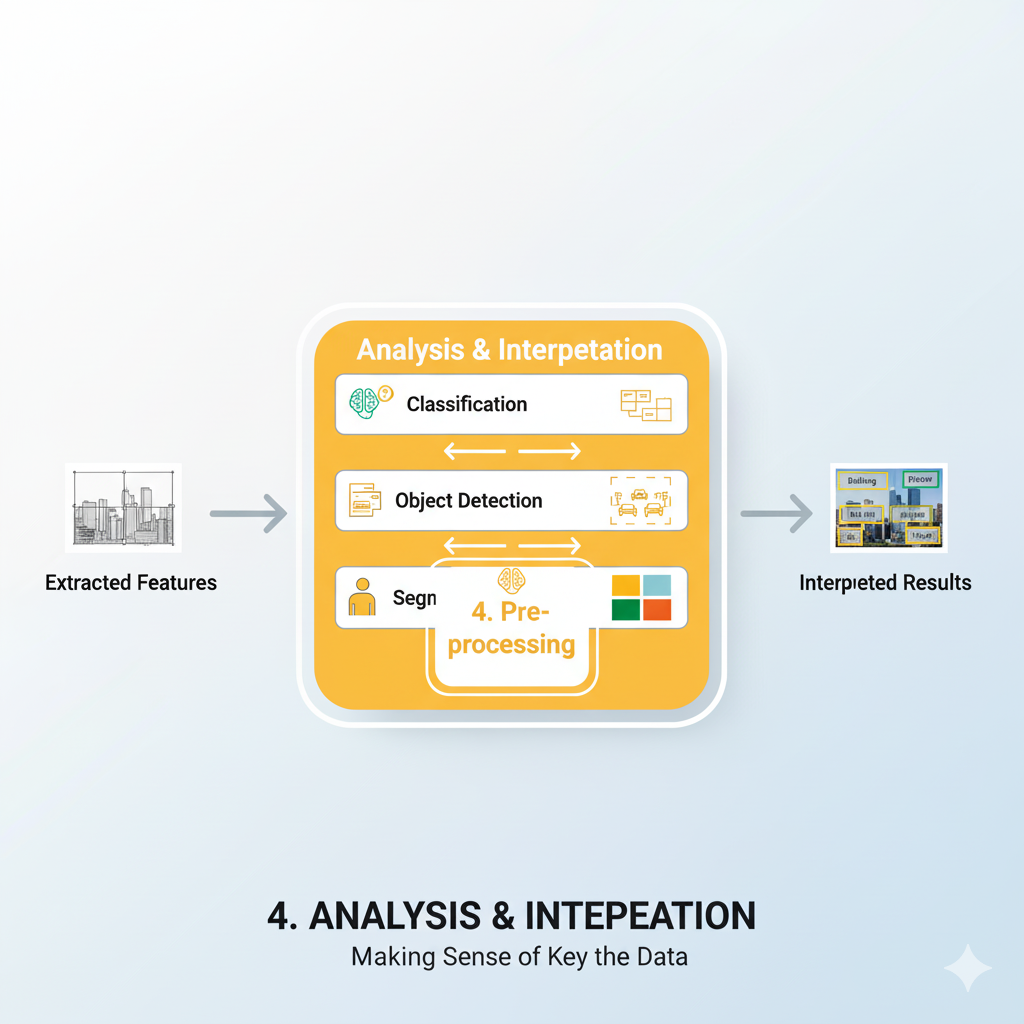
Finally, we package our extracted geometries and any associated data into a standard format.

• Create Vector Data: We create a GeoJSON or Shapefile where each “feature” (e.g., a country) has a geometry (the polygon we extracted) and properties (like the country name, which we might get from a separate step like OCR).
• Add Attributes: If the map had labels (e.g., city names, values in a choropleth map), you could use Optical Character Recognition (OCR) tools like Tesseract to read them and link them to the corresponding shapes.

Final Output: A countries.geojson file that you can load into QGIS, plot with Python, or analyze for area, perimeter, proximity, etc.

A Simple Python Example with OpenCV

Photo by Ilya Pavlov on Unsplash

This code demonstrates the core concept for a perfectly clean, simple map image.

import cv2
import numpy as np
import geojson
from rasterio.transform import from_bounds

# Step 1: Preprocessing
image = cv2.imread('simple_world_map.png')
gray = cv2.cvtColor(image, cv2.COLOR_BGR2GRAY)
_, binary = cv2.threshold(gray, 127, 255, cv2.THRESH_BINARY)

# Step 2: Feature Extraction
contours, _ = cv2.findContours(binary, cv2.RETR_EXTERNAL, cv2.CHAIN_APPROX_SIMPLE)

# Assume we know the geographic bounds of our map image
# This is a CRITICAL step that requires manual input or knowledge of the map.
pixel_left, pixel_right = 0, binary.shape[1]  # Image width
pixel_bottom, pixel_top = 0, binary.shape[0]  # Image height
geo_left, geo_bottom = -180, -90   # Longitude, Latitude
geo_right, geo_top = 180, 90

transform = from_bounds(geo_left, geo_bottom, geo_right, geo_top, binary.shape[1], binary.shape[0])

features = []
for contour in contours:
    # Simplify the contour
    epsilon = 0.002 * cv2.arcLength(contour, True)
    approx = cv2.approxPolyDP(contour, epsilon, True)

    # Step 3: Georeferencing - Convert pixels to geo coordinates
    geo_coords = []
    for point in approx:
        x_pixel, y_pixel = point[0]
        # Use the affine transform
        lon, lat = transform * (x_pixel, y_pixel)
        geo_coords.append((lon, lat))

    # Create a GeoJSON feature (assuming it's a polygon)
    if len(geo_coords) > 2:  # A polygon needs at least 3 points
        polygon = geojson.Polygon([geo_coords])
        features.append(geojson.Feature(geometry=polygon))

# Step 4: Data Structuring
feature_collection = geojson.FeatureCollection(features)

# Save the actionable data!
with open('extracted_map_data.geojson', 'w') as f:
    geojson.dump(feature_collection, f)

print("Done! Map has been 'unflattened' to extracted_map_data.geojson")

Challenges and Advanced Techniques

• Noisy or Complex Images: Requires more sophisticated preprocessing (e.g., edge detection with cv2.Canny).
• Overlapping Features: Contour detection might need to be hierarchical (cv2.RETR_TREE).
• Text and Labels: Integrating OCR (Tesseract) to extract labels and associate them with the correct shape is a non-trivial challenge.
• Handling Distortion: For non-planar maps (e.g., a photo of a globe), more complex reprojection is needed.

.

🗺️ The Magic of “Unflattening” Maps

Unflattening is the process of converting 2D images into a more informative, structured, or 3D-like map.

Using only the image:

Terrain shading → estimated slope

Color variations → elevation changes

Shadows → depth inference

Natural curves → topology approximation

These techniques power:

✔ 3D terrain reconstruction ✔ Smart GIS layer generation ✔ Autonomous navigation systems ✔ Game map generation ✔ Historical map preservation

Real Example: Elevation From Shaded Relief

Even a simple grayscale relief image contains hidden depth information.

Using algorithms like:

Shape-from-shading

Gradient mapping

Photometric stereo

You can generate:

Height maps

Slope maps

3D mesh surfaces

This allows terrain reconstruction with zero external data — only the image is used.

⚙️ The Tech Stack Behind the Magic

Here are common tools used in image-based map reconstruction:

• OpenCV — edge, contour, thresholding
• scikit-image — transformations, segmentation
• NumPy — pixel-level computation
• TensorFlow/PyTorch — enhancement, super-resolution
• QGIS + Python — map export and visualization
• Blender — 3D mesh creation from height maps

You can build powerful “data-less” mapping pipelines using these open-source tools.

Conclusion

“No Data, No Problem” is a powerful mindset. By applying image processing techniques, we can liberate data trapped in static images. This allows us to:

• Digitize historical maps for temporal analysis.
• Extract data from published charts and graphs for re-analysis.
• Create geospatial datasets from screenshots when an API is unavailable.
• Automate the conversion of large collections of map images.

The journey from a simple image to a structured, queryable dataset is a perfect blend of computer vision and data science, turning pixels into profound insights.