Visualising Chaos using RK4

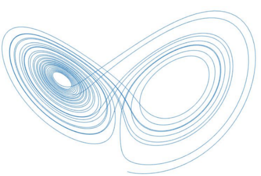
The Lorentz Attractor

TL;DR: The Lorenz system is a set of differential equation that describe a simplified mathematical model of atmospheric convection. Calculating solutions of the Lorenz system using the fourth-order Runge-Kutta algorithm (RK4), it is clear that the system is sensitive to changes in its initial conditions in certain regimes of the parameters; the system exhibits chaotic behaviour with (Prandtl number) a ~ 10, (Rayleigh number) r ~ 28, and (geometric factor) b ~ 8/3. In the chaotic regime we observe the Lorenz attractor. Project code is written in MATLAB and is available here.

Introduction: Lorenz System

The Lorenz equation are three ordinary differential equations that form the Lorenz model. The Lorenz equation of the time-dependent variables are:

where a, r, and b are constants.

These equations can be used as a simplified model of atmospheric convection, with each variable describing properties of the fluid in the Rayleigh-Bénard experiment, and they can be derived from the Navier-Stokes equations, the equation for heat conduction and the continuity equation [1]. Physically, y₁ is proportional to the rate of convection, y₂ to the temperature difference between currents, and y₃ is the temperature difference between the top and the bottom of the fluid, where a is the Prandtl number, r is the Rayleigh number, and b is a geometric factor [2].

The set of equations has three stationary solutions:

The approach to these solutions from an arbitrary starting point and dependent on the regime of r [3].

1. If r < 1 the only real stationary point is the origin.
2. If r > 1 all three stationary points exist. However, the origin is unstable and so you will never reach it unless you start exactly on it. As r increases, there is a higher degree of uncertainty in the system.

Additionally, if r > 1 but less that about 24 the system will converge to one of the two stationary points not found at the origin. In contrast, if r > 1 but greater than about 24, the system will not converge to either solution and will move between the two fixed points in space (the behaviour is bounded but non-periodic).

“Mann muss noch Chaos in sich haben, um einen tanzenden Stern gebären zu können.”

(One must still have chaos in oneself to be able to give birth to a dancing star)

- Friedrich Nietzsche (from “Thus Spoke Zarathustra”)

Introduction: RK4

The Lorenz equations are coupled first order differential equation and numerical solutions are much easier to obtain than attempts to solve analytically through decouple the solutions or particular integrals and complementary functions. Runge-Kutta methods are iterative methods of approximately solving ordinary equations using small time steps. The Runge-Kutta method implemented in this program was the fourth-order method (RK4). The Lorentz equations are in the form,

Defining a small time interval δt, the value of the yᵢ can be iteratively calculated at time steps of δt. Referring to the mth intermediate point in our calculation as yᵢ,ₘ and fᵢ,ₘ, the RK4 iteration steps are:

The values yᵢ,₄ then become yᵢ,₀ in the next step and the value of yᵢ,ₙ, where n = 4m, corresponds to the value of yᵢ at time, t = mδt. The initial conditions of the system yᵢ,₀ and the parameters of the system, a, b and r can be varied. Although faster methods exist, Runge-Kutta methods nearly always work and hence are often used to produce a numerical solution [4]. Runge-Kutta algorithms are derived from Simpson’s rule and use varying subintervals depending on their order; the fourth order algorithm gives the best balance between accuracy and computational effort [5]. These algorithms are better approximations of solutions than Euler’s method due to the use of higher order terms which reduces truncation error, but they require more computational power.

Different Regimes of r

We fix the values of the parameters a = 10 and b = 8/3. Also, to compare different regimes we fix the initial conditions y₁,₀ = 1, y₂,₀ = 2 and y₃,₀ = 3 and the solutions are evaluated over n = 500 time steps, δt = 0.05.

r < 1

Setting r = 0, from Figure 1(a), we observe that the values of y₁, y₂ and y₃ converge to zero, which we expect since the only real stationary point in this regime is the origin. Figure 1(b) shows the relation between variables y₂ and y₃; their behaviour towards converging at the origin is non-chaotic.

1 < r < 24

Setting r = 15, from Figure 2(a), we observe that the values of y₁, y₂ and y₃ converge to one of the solutions, not including the origin, unless the initial conditions start at the origin since it is unstable. Figure 2(b) shows this convergence is a reached by spiralling around the solution.

r > 24

Setting r = 30, from Figure 3(a), we observe that the values of y₁, y₂ and y₃ do not converge to one of the solutions, but instead wanders between the two solutions that are not the unstable origin. Figure 3(b) shows this convergence is a reached by spiralling around the solution.

This is a strange attractor, since the solutions are bounded but non-periodic. Plotting all three coordinates against each other, a more intuitive image of the Lorentz attractor can be viewed as in Figure 4. Reducing the step size, δt, to 0.0001, we obtain the smoother Lorenz attractor at the top of the article.

Visualising Chaotic Behaviour: ‘the weather forecasting’ phenomena

In the r > 24 regime, we observe what seems to be chaotic behaviour. To analyse this behaviour we fix the values of the parameters a = 10, b = 8/3 and r = 28, but slightly change the initial conditions y₁,₀, y₂,₀ and y₃,₀. As before, the solutions are evaluated over n = 500 time steps, δt = 0.05. Initially, we set the initial conditions y₁,₀ = 4, y₂,₀ = 5and y₃,₀ = 6, which we call these the real conditions. The time-evolution of the variables are compared to initial conditions y₁,₀ = 4.01, y₂,₀ = 5.01 and y₃,₀ = 6.01, which we call a ‘small measurement error’.

Focusing on the time-evolution of y₁, Figure 5 shows that the slight change in initial conditions leads to a similar initial time evolution. However, after a short period of time the solutions separate and begin to wander about the two solutions following different paths. This demonstrates deterministic chaotic behaviour, since the present determines the future but the approximate present does not approximately determine the future. Since, weather systems can be approximated by the Lorentz model this demonstrates the difficulties of predicting the weather; small measurement errors will lead to vastly different outcomes.

Final Comments

The Lorentz system demonstrates chaotic behaviour in the regime r > 24, since a small change in the initial conditions of the system drastically changes the time-evolution of the system. The Lorentz attractor is observed, since the system is bounded by two solutions, but does not converge to either. In the approximately the regime 1 < r < 24, the system will converge to one of the two solutions, which are not the origin, depending upon initial conditions. In the regime, r < 1, the system will converge to the solution at the origin.

The RK4 method offers a clear visualisation of the chaotic behaviour observed. However, since the RK4 method is an iterative method it propagates error. This is particularly unhelpful when studying chaos as the system is sensitive to small changes and therefore the numerical solution obtained by the RK4 method is likely to be vastly different from the actual solution after a long period of time; a small local error develops into a large global error. Another disadvantage in my ODE solver program was the use of equally spaced time intervals as at turning points the RK4 method is more inaccurate. Combing the RK4 method with intelligent adaptive step-size routine would increase the accuracy of the solution; MatLab has an inbuilt ode45 function that uses RK4 with changing time-steps. For systems with a large numbers of coupled equations, this adaptive step-size is particularly important. The ODE solver is extremely versatile and slight modifications to the program allow the higher order ODEs to be solved, such as a damped oscillator.

**Code Repository**

[1] Schuster H. G. (1988). Deterministic chaos: an introduction, 2nd Ed. Darmstadt: betz-druck gmbh, p223–225.

[2] https://mathworld.wolfram.com/LorenzAttractor.html

3] (2018). Lorentz Attractor [Accessed 24 January 2020] Available at: https://wwwteaching.physics.ox.ac.uk

[4] Press W. H. et al. (2007). Numerical Recipes: the Art of Scientific Computing, 3rd Ed. Cambridge: Cambridge University Press, p908.

[5] O’Hare A. (2005). Numerical Methods for Physicists, Oxford Physics, p69.