🔥 BiFormer Reshapes Visual Attention with “Bi-Level Routing”: Shaking Up SOTA at Lower Computational Cost

— — Decoupling how Bi-Level Routing Attention enables Vision Transformers to “look less and think more”

📌 Introduction: When Transformers Meet the “Attention Tax”

Over the past few years, the Vision Transformer (ViT) has practically taken over the computer vision landscape. From image classification to object detection, semantic segmentation, and instance segmentation, Transformer architectures have repeatedly pushed the boundaries of visual tasks thanks to their global receptive fields, parallel computing capabilities, and data-driven flexibility.

Yet, in this era where “attention is king,” a notorious pain point continues to haunt researchers:

The computational complexity and memory footprint of Vanilla Attention scales at $O(N²)$, where $N$ is the number of tokens.

What does this mean in practice? If a $224 \times 224$ image is split into $16 \times 16$ patches, we get $196$ tokens — requiring a $196 \times 196$ affinity matrix. But when resolution scales up to $1024 \times 1024$ or higher, the number of tokens explodes, causing the computational load to climb quadratically. This is the dreaded “attention tax.”

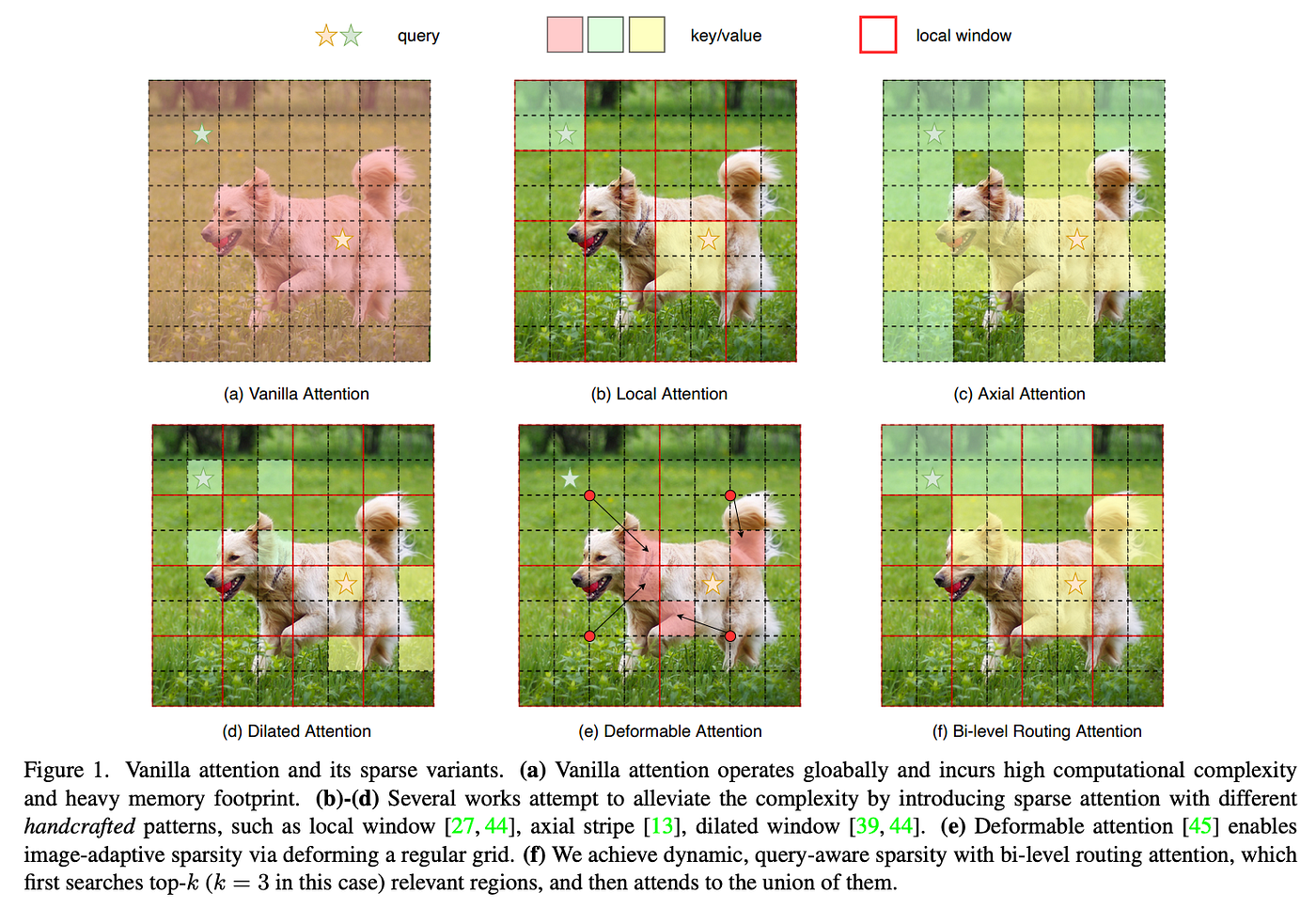
To offset this cost, the academic community has tried numerous workarounds: local windows (Swin Transformer), criss-cross windows (CSWin), dilated windows (Dilated Attention), and axial stripes (Axial Attention).

However, these methods share a common limitation: their sparsity patterns are “handcrafted” or “query-agnostic.” In other words, every query is forced to share the exact same set of key-value tokens regardless of its content.

The research team behind BiFormer noticed a counter-intuitive phenomenon:

💡 Queries from different semantic regions actually focus on vastly different key-value pairs!

This observation sparked their core insight: sparsity shouldn’t be a “one-size-fits-all” constraint. Instead, it should be dynamic, query-aware, and content-dependent. This led to the creation of BiFormer, a novel Vision Transformer powered by its proprietary Bi-Level Routing Attention (BRA), which achieves state-of-the-art (SOTA) performance across multiple vision tasks with significantly lower computational overhead.

🧠 Part 1: The Collective Dilemma of Existing Sparse Attention

Before diving into BiFormer, it helps to understand where existing sparse attention mechanisms fall short.

1.1 Handcrafted Sparsity Patterns

Swin Transformer’s shifted window attention is an industry classic. It divides a feature map into non-overlapping $7 \times 7$ windows, computes self-attention within those windows, and uses a shifting mechanism to let adjacent windows communicate. While clean and highly efficient, its receptive field is naturally constrained — an individual token cannot directly “see” distant information.

Subsequent frameworks like CSWin and CrossFormer expanded the receptive field using criss-cross or axial windows, but these remain predefined, static patterns that fail to exploit the image’s inherent semantic layout.

1.2 Adaptive Sparse Approaches

Methods like DAT (Deformable Attention Transformer) and DPT attempt to let models adaptively select key-value tokens. However, they run into a fundamental paradox:

• To achieve true query-aware selection, they must either calculate all query-key affinities (which defeats the purpose by spiking complexity),
• Or use local contexts to predict offsets (similar to Deformable Convolutions), which struggles to model long-range dependencies.

1.3 Quad-Tree Attention: Elegance at a Price

Another branch of work, like QuadTree Attention, builds token pyramids to compute attention at different granularities. While theoretically elegant, it comes with heavy real-world costs:

• Deep recursion severely compromises parallelism.
• It relies heavily on sparse matrix multiplication, which is notoriously inefficient on modern GPUs.
• As a result, actual throughput falls short of expectations.

1.4 Core Pain Point Summary

Existing methods are either static (handcrafted), query-agnostic (sharing tokens across all queries), or computationally unfriendly (relying on GPU-inefficient sparse matrices). The authors of BiFormer pointed out the core flaw bluntly:

🚨 Forcing all queries to attend to the same set of key-values is fundamentally sub-optimal.

This exact realization served as the logical starting point for BiFormer.

🌟 Part 2: Bi-Level Routing Attention (BRA) — Core Idea

2.1 A Useful Analogy

Imagine you are looking for reference materials in a massive university library. Traditional Vanilla Attention is like checking every single book on every shelf to see if it’s relevant — exhausting and impractical. Static Sparse Attention is like restricting yourself to just one pre-assigned shelf — efficient, but you’ll likely miss crucial books stored elsewhere.

BiFormer’s approach is different: It quickly skims the labels of each bookshelf (coarse-grained, region-level routing) to pinpoint the few shelves most likely to contain what you need. Then, it dives deep into only those selected shelves to read the specific books (fine-grained, token-level attention).

This is Bi-Level Routing — filter broadly first, select precisely second.

2.2 The Overall BRA Flow

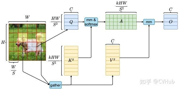
The design philosophy behind BRA is simple: filter out the most irrelevant key-value pairs at the lowest possible cost. The pipeline works as follows:

1. Region Partitioning: The input feature map $X \in \mathbb{R}^{H \times W \times C}$ is divided into $S \times S$ non-overlapping regions, where each region contains $\frac{HW}{S²}$ tokens.
2. Linear Projection: $Q$, $K$, and $V$ tensors are derived via linear projections within each region.
3. Region-Level Routing (Graph Construction & Pruning):

• Compute the average of $Q$ and $K$ within each region to derive region-level queries ($Q_r$) and region-level keys ($K_r$).
• Compute a region-to-region affinity matrix ($A_r$) via matrix multiplication.
• Apply a Top-$k$ operation to keep only the $k$ most relevant routing neighbors for each region, generating a routing index matrix ($I_r$).

4. Token-Level Attention:

• Gather the key-value pairs from the regions indexed by $I_r$.
• Run standard token-to-token attention over this pruned union of routed regions.
• Introduce a local context enhancement term (via a $5 \times 5$ depthwise convolution) to smooth the output.

The entire process is neatly summarized by the authors’ PyTorch-style pseudocode:

# Python

# 1. Patchify into S² regions
x = patchify(input, patch_size=H//S)
# 2. Linear projection
query, key, value = linear_qkv(x).chunk(3, dim=-1)
# 3. Region-level query & key (via region averaging)
query_r, key_r = query.mean(dim=1), key.mean(dim=1)
# 4. Region-level affinity graph
A_r = mm(query_r, key_r.transpose(-1, -2))
# 5. Top-K routing index
I_r = topk(A_r, k).index
# 6. Gather routed key-values
key_g = gather(key, I_r)
value_g = gather(value, I_r)
# 7. Token-level attention + local enhancement
output = bmm(softmax(bmm(query, key_g.transpose(-2,-1))), value_g) + dwconv(value)

2.3 Why is this Design so Clever?

• Brilliant Point 1: Coarse-to-Fine Hierarchical Filtering The authors mathematically prove in their appendix that maximizing token-level affinity across two regions is bounded by maximizing the affinity of their region-average vectors. This means using region-level averages for coarse filtering is not just computationally cheap, but theoretically sound.
• Brilliant Point 2: GPU-Friendly Dense Matrix Multiplications Routed regions are scattered across different spatial coordinates, which theoretically calls for sparse matrix operations. However, modern GPUs rely on coalesced memory access, making random sparse lookups incredibly slow. BiFormer bypasses this by using a gather operation to collect scattered key-values into a contiguous tensor first, allowing the model to run standard, highly optimized dense matrix multiplications. This single choice bridges the gap between theoretical elegance and engineering utility.
• Brilliant Point 3: Dynamic and Query-Aware Instead of forcing all queries to share a static set of tokens, each query determines its own routing paths independently. This allows the model to automatically decide where to look based on contextual content.

📐 Part 3: Complexity Analysis — Why BRA is Incredibly Efficient

Complexity is the ultimate benchmark for any attention mechanism. Let’s look at how different architectures scale:

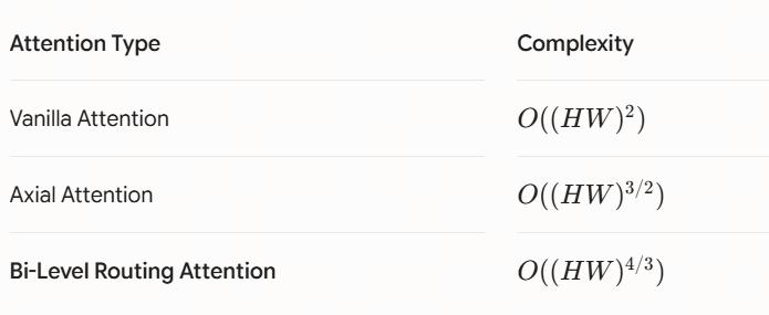
Attention TypeComplexityVanilla Attention$O((HW)²)$Axial Attention$O((HW)^{3/2})$Bi-Level Routing Attention$O((HW)^{4/3})$

The complexity of BRA is derived from three main operations:

• Linear Projection: $3HWC²$
• Region-Level Routing: $2(S²)²C$
• Token-Level Attention: $2HW \cdot k \cdot \left(\frac{HW}{S²}\right) \cdot C$

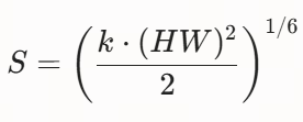
By applying the AM-GM (Arithmetic Mean-Geometric Mean) inequality, the authors prove that when the region partition factor $S$ matches:

$$S = \left(\frac{k \cdot (HW)²}{2}\right)^{1/6}$$

the total computational cost of BRA reaches its optimal theoretical lower bound of $O((HW)^{4/3})$.

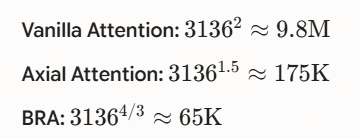
To put this into perspective, let’s look at an input size of $HW = 56 \times 56 = 3136$:

Vanilla Attention: 3136² = 9.8M, Axial Attention: 3136^{1.5} = 175K, BRA: 3136^{4/3} = 65K

📉 The computational footprint of BRA is two orders of magnitude lower than Vanilla Attention, and significantly lower than Axial Attention!

However, the authors transparently note that choosing $S$ and $k$ involves a few real-world engineering trade-offs:

• $S$ must be a clean divisor of the input resolution to avoid messy padding.
• Dense prediction tasks require a larger $S$ to balance the overhead between routing and token attention.
• $k$ needs to scale up progressively across deeper stages as regions shrink.

🏗️ Part 4: The Overall BiFormer Architecture

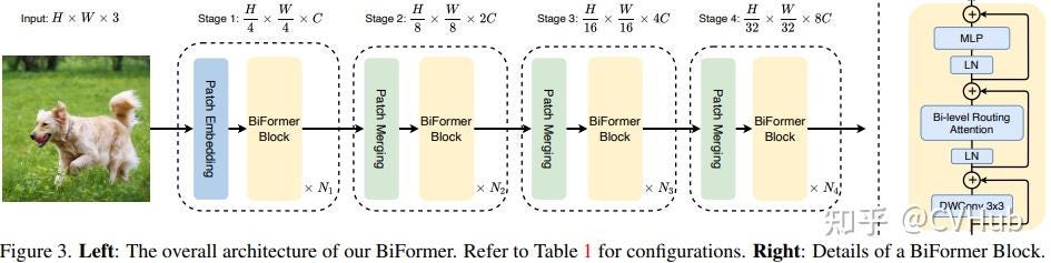
With BRA acting as the primary building block, constructing a complete Vision Transformer becomes straightforward. BiFormer adopts a standard four-stage pyramid structure (consistent with Swin and CSWin) to facilitate easy comparison:

4.1 Framework Breakdown

• Stage 1: Uses an overlapping patch embedding to preserve higher spatial resolutions.
• Stages 2–4: Employs patch merging modules to downsample feature maps while doubling channel dimensions.
• Each stage consists of a series of stacked BiFormer Blocks.

4.2 Anatomy of a BiFormer Block

Every block integrates three complementary steps:

• $3 \times 3$ Depthwise Convolution: Implicitly encodes relative position information (drawing inspiration from ConvNeXt and UniFormer).
• BRA Module: Captures dynamic, cross-location dependencies.
• 2-layer MLP (expansion ratio = 3): Handles position-wise embedding transformations.

🧩 This hybrid “Conv + Attention + MLP” layout follows a highly practical engineering philosophy: let convolutions handle local patterns, and let attention capture global dependencies.

4.3 Model Scaling Specifications

ModelChannelsBlocks per StageParamsFLOPsBiFormer-T64[2, 2, 8, 2]13M2.2GBiFormer-S64[4, 4, 18, 4]26M4.5GBiFormer-B96[4, 4, 18, 4]57M9.8G

The top-$k$ routing values are configured as [1, 4, 16, S²] respectively (the final stage defaults to full attention because the resolution is highly compact). For downstream tasks, $S=7$ for classification, $S=8$ for semantic segmentation, and $S=16$ for object detection.

📊 Part 5: Experimental Results — Outperforming the Field

5.1 ImageNet-1K Image Classification

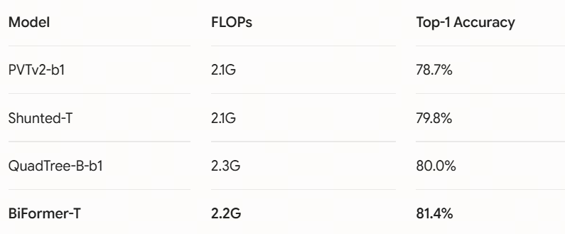
Evaluated on the standard ImageNet-1K benchmark ($300$-epoch training, no external data), BiFormer demonstrates exceptional efficiency:

Small Models (~2G FLOPs):

ModelFLOPsTop-1 AccuracyPVTv2-b12.1G78.7%Shunted-T2.1G79.8%QuadTree-B-b12.3G80.0%BiFormer-T2.2G81.4%

🏆 BiFormer-T achieves 81.4% accuracy at just 2.2G FLOPs, outperforming QuadTree-b1 by 1.4% with less compute!

Medium Models (~4G FLOPs):

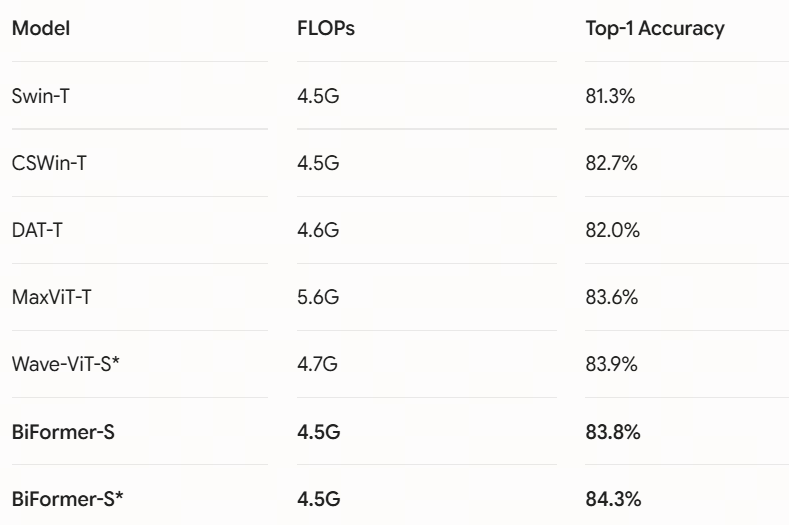
ModelFLOPsTop-1 AccuracySwin-T4.5G81.3%CSWin-T4.5G82.7%DAT-T4.6G82.0%MaxViT-T5.6G83.6%Wave-ViT-S4.7G83.9%BiFormer-S4.5G83.8%BiFormer-S4.5G84.3%

(Note: * indicates the inclusion of Token Labeling).

Large Models (~10G FLOPs):

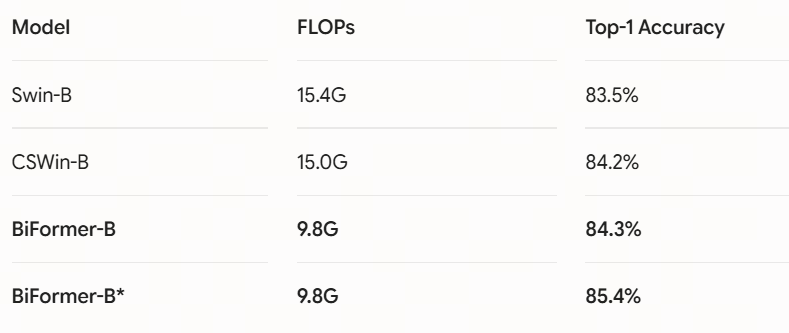
ModelFLOPsTop-1 AccuracySwin-B15.4G83.5%CSWin-B15.0G84.2%BiFormer-B9.8G84.3%BiFormer-B9.8G85.4%*

🚀 BiFormer-B beats 15G-level models like Swin-B and CSWin-B while using only 9.8G FLOPs and a compact 57M parameter footprint.

5.2 COCO Object Detection and Instance Segmentation

BiFormer carries over its performance gains to dense downstream tasks like COCO 2017:

RetinaNet (1× schedule):

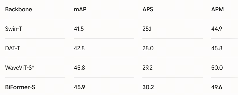
BackbonemAPAPS​APM​APL​Swin-T41.525.144.955.5DAT-T42.828.045.857.8WaveViT-S45.829.250.060.8BiFormer-S45.930.249.661.7*

Mask R-CNN (1× schedule):

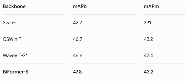
BackbonemAPbmAPmSwin-T42.239.1CSWin-T46.742.2WaveViT-S46.642.4BiFormer-S47.843.2*

🔍 Crucially, BiFormer shines in detecting small objects ($AP_S$ of 30.2 vs Swin-T’s 25.1). The authors attribute this to BRA using sparse sampling rather than aggressive downsampling, which preserves critical fine-grained structural details.

5.3 ADE20K Semantic Segmentation

On the challenging ADE20K dataset, BiFormer scales cleanly across both Semantic FPN and UperNet frameworks:

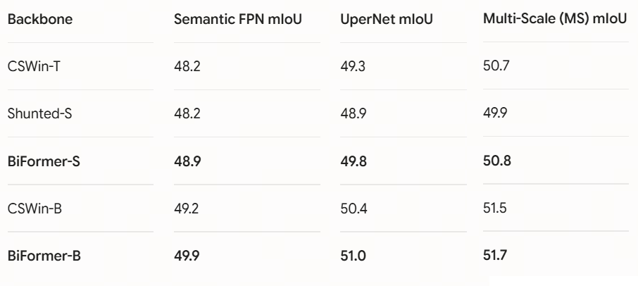
BackboneSemantic FPN mIoUUperNet mIoUMulti-Scale (MS) mIoUCSWin-T48.249.350.7Shunted-S48.248.949.9BiFormer-S48.949.850.8CSWin-B49.250.451.5BiFormer-B49.951.051.7

🔬 Part 6: Ablation Studies — What Makes BRA Work?

6.1 BRA vs. Other Sparse Attention Mechanisms

To isolate the impact of BRA, the authors ran a controlled experiment keeping the Swin-T baseline architecture identical, swapping out only the attention module:

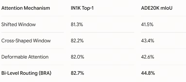
Attention MechanismIN1K Top-1ADE20K mIoUShifted Window81.3%41.5%Cross-Shaped Window82.2%43.4%Deformable Attention82.0%42.6%Bi-Level Routing (BRA)82.7%44.8%

🏅 BRA leads the runner-up by 0.5% in classification and a substantial 1.4% in segmentation, proving that content-aware dynamic routing delivers clear benefits.

6.2 Structural Evolution

Tracing the modifications from a vanilla Swin-T layout to BiFormer-S reveals where the gains come from:

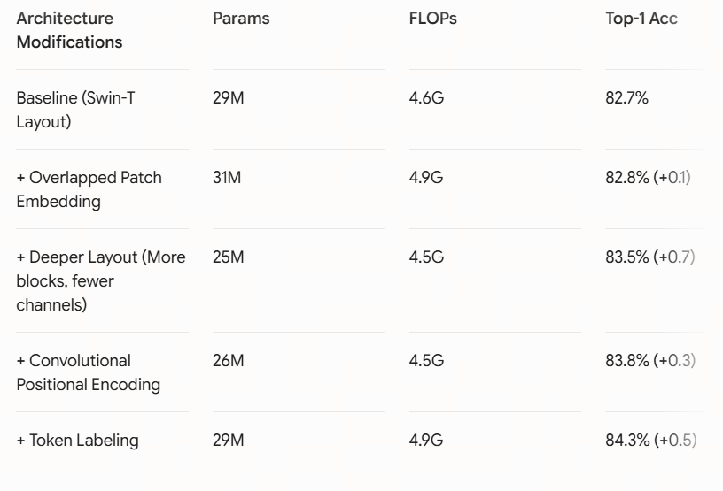
Architecture ModificationsParamsFLOPsTop-1 AccBaseline (Swin-T Layout)29M4.6G82.7%+ Overlapped Patch Embedding31M4.9G82.8% (+0.1)+ Deeper Layout (More blocks, fewer channels)25M4.5G83.5% (+0.7)+ Convolutional Positional Encoding26M4.5G83.8% (+0.3)+ Token Labeling29M4.9G84.3% (+0.5)

💡 An interesting takeaway: Simply opting for a “deeper but narrower” topology (more blocks, fewer channels) accounted for a $+0.7\%$ performance bump — a structural refinement often overlooked in architectural papers.

6.3 A Counter-Intuitive Discovery

During hyperparameter tuning for $S$ and $k$, the authors stumbled upon a fascinating quirk: increasing the number of attended tokens sometimes hurts model accuracy.

SkAttended TokensAccuracySpeed7[1,4,16,49][64,64,64,49]82.7%522 im/s7[1,2,8,32][64,32,32,32]82.4%563 im/s[8,4,2,1][2,2,2,1][98,98,98,49]82.3%606 im/s

🤔 This suggests that explicit sparsity constraints function as a form of regularization. By forcing the model to ignore irrelevant regions, it avoids over-fitting to background noise.

6.4 Visualization: What Does BiFormer Actually Focus On?

Visualizing the routing paths on COCO images reveals highly rational, content-aware attention maps:

• When a query token sits on a building, the routing mechanism exclusively activates other building regions across the image.
• When the query is on a tree, the attention map highlights scattered foliage regions.
• In indoor scenes, placing a query on a computer mouse instantly routes attention to the keyboard, monitor, and PC tower — connecting semantically related but spatially disconnected objects.

🧪 Part 7: Throughput Analysis — Real-World Trade-offs

BiFormer is highly optimized, but it isn’t without its caveats. The authors include an honest breakdown of hardware throughput metrics measured on a Tesla V100 GPU (using a batch size of 128 at $224 \times 224$ resolution):

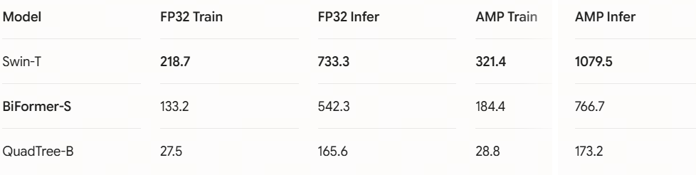
ModelFP32 TrainFP32 InferAMP TrainAMP InferSwin-T218.7733.3321.41079.5BiFormer-S133.2542.3184.4766.7QuadTree-B27.5165.628.8173.2

⚠️ BiFormer’s training throughput is roughly 30% lower than Swin-T, and its inference throughput drops by about 40%. This is due to the sequential overhead of running the routing logic, managing kernel launches, and executing tensor gathers in memory.

That said, BiFormer runs 3 to 6 times faster than QuadTree, and the authors point out that these memory bottlenecks can be substantially mitigated in production via custom GPU kernel fusion and optimized CUDA implementations.

💡 Part 8: Broad Takeaways from BiFormer

8.1 The Philosophy of “Less is More”

BiFormer teaches us an important lesson about visual processing: not all patches deserve equal attention. Rather than forcing a query to scan the entire image canvas passively, letting each query actively elect its target regions serves as a layer-level “early exit.” This drops FLOP counts while cleaning up ambient background noise.

8.2 The Coarse-to-Fine Paradigm

The two-stage framework (coarse region routing followed by fine token attention) closely mirrors human visual cognition. When humans look at an environment, we map out the macro-layout first before focusing our gaze on specific items of interest. This hierarchical approach offers a powerful reference design for future efficient architectures.

8.3 Hardware-First Engineering Mindset

What makes BiFormer outstanding is its rejection of purely theoretical elegance in favor of practical hardware compatibility. Choosing a gather step followed by standard dense matrix multiplications bypasses the heavy latency penalties typical of sparse GPU operations. Designing algorithms around hardware constraints is a crucial practice for deployable AI.

📝 Part 9: Limitations and Future Horizons

The paper notes a few key areas for improvement:

• Runtime Overhead: The memory gather and kernel orchestration operations limit raw throughput relative to purely local window models like Swin.
• Optimization Potential: Writing dedicated CUDA operators and utilizing advanced graph compilers could drastically narrow the throughput gap.
• Extensions: Applying dynamic bi-level routing to alternative domains, such as multi-modal learning or video processing, remains a highly promising avenue.

🎬 Conclusion

BiFormer’s main contributions boil down to three points:

• Introduces BRA: Leverages bi-level routing to realize a dynamic, query-aware sparse attention mechanism.
• Improves Algorithmic Scaling: Drops complexity down to $O((HW)^{4/3})$, well below standard self-attention.
• Sets New Benchmarks: Delivers exceptional accuracy gains across ImageNet, COCO, and ADE20K while maintaining a lower FLOP count.

BiFormer reminds us of an intuitive truth in computer vision engineering: sometimes, looking at less helps you see much clearer.

📚 Paper Reference

• Title: BiFormer: Vision Transformer with Bi-Level Routing Attention
• Authors: Lei Zhu, Xinjiang Wang, Zhanghan Ke, Wayne Zhang, Rynson Lau
• Paper Link: arXiv:2303.08810
• Official Code: GitHub — rayleizhu/BiFormer