Time Series 3 — Stationarity vs Non Stationarity, Strict and Weak Stationarity, ADF and KPSS Test

Before building many classical forecasting models such as ARIMA, one concept becomes extremely important: stationarity.

In simple terms, stationarity describes whether the statistical properties of a time series remain constant over time.

Many time series models assume that the data does not change its behavior over time. If the mean, variance, or relationships between values keep changing, those models struggle to learn meaningful patterns.

What is Stationarity?

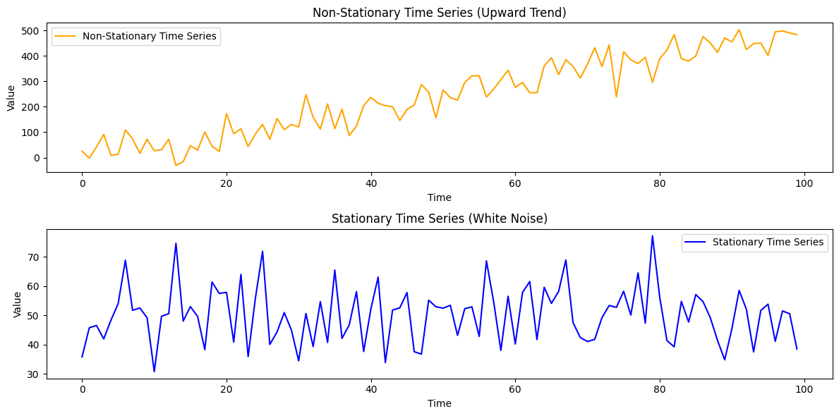
A time series is stationary if its statistical properties remain constant over time.

These properties include:

• Mean
• Variance
• Autocorrelation structure

This means:

• The average value (mean) stays roughly the same.
• The spread of values (variance) stays similar.
• The relationship between past and future values remains consistent.

If these remain stable, the data behaves similarly at different time periods.

If any one of these properties changes over time, the series is considered non-stationary

Example of Stationary Data

Imagine temperature readings inside a controlled room.

The temperature fluctuates slightly but stays around the same value.

Example of Non-Stationary Data

Now consider a dataset with a trend.

Example: company sales growing every month.

Strict Stationarity

Strict stationarity means, the statistical properties remains constant over time

The best example of strict stationarity is IID (Independent and Identically Distributed) noise. Imagine rolling a fair die every hour:

• The probability of rolling a 4 is always 1/6
• The average will always be 3.5.
• The “rules” never change.

Strict stationarity says:

If we take any group of values in the time series, their joint behavior should stay the same over time.

Example groups:

Early time:

(Sales₁, Sales₂)

Later time:

(Sales₁₀, Sales₁₁)

Strict stationarity requires:

The relationship between these pairs should look statistically the same.

What do we mean by “Covariance depends only on lag, not time” here?

Step 1: What covariance means here

Covariance in time series measures how two values move together.

Example:

• If sales today are high and tomorrow is also high → positive covariance
• If sales today are high but tomorrow is low → negative covariance

If the covariance between Xt and X{t+1} is positive and constant, it just means that if today is above the average, tomorrow is also likely to be above the average. It doesn’t mean tomorrow has to be higher than today. It just has to be on the same “side” of the mean.

A Simple Analogy: The Thermostat

• Stationary: A room with a thermostat set to 22°C. The temperature wiggles between 21.5°C and 22.5°C all day. The “rules” (mean = 22, variance = small wiggle) never change. The relationship between the temp at 1:00 PM and 1:01 PM is the same as at 4:00 PM and 4:01 PM.
• Non-Stationary (Increasing): You turn the heater on and leave it. The temperature goes 22, 23, 24, 25… The “mean” is moving. This is a trend, and it violates stationarity.

So covariance tells us how two time points are related.

Why Stationarity Matters

Many forecasting models assume that past patterns will continue into the future.

If the statistical properties of the data keep changing, the model cannot learn stable relationships.

For example:

Suppose we train a model on sales data.

Year 1 average sales = 100 Year 5 average sales = 600

The model learns patterns based on earlier data, but those patterns no longer represent the future.

This leads to poor predictions.

Models that require stationary data include:

• ARIMA
• SARIMA
• AR models
• MA models

These models rely heavily on autocorrelation (Autocorrelation simply means how much a value in a time series is related to its own past values), which behaves properly only when the data is stationary.

Augmented Dickey-Fuller (ADF) Test

The ADF test is one of the most commonly used statistical tests for stationarity.

It checks whether the time series contains a unit root.

A unit root indicates non-stationarity.

Hypothesis

Null Hypothesis (H₀): The series has a unit root → data is non-stationary

Alternative Hypothesis (H₁): The series is stationary

Python example:

from statsmodels.tsa.stattools import adfuller

result = adfuller(data)
print("ADF Statistic:", result[0])
print("p-value:", result[1])

Interpretation

If the p-value is less than 0.05

We reject the null hypothesis.

This means the data is stationary.

If the p-value is greater than 0.05

We fail to reject the null hypothesis.

This suggests the data is non-stationary.

KPSS Test

The KPSS test approaches stationarity from the opposite direction.

Instead of checking for a unit root, it checks whether the series is stationary around a deterministic trend.

Hypothesis

Null Hypothesis (H₀): The series is stationary

Alternative Hypothesis (H₁): The series is non-stationary

Python example:

from statsmodels.tsa.stattools import kpss

statistic, p_value, lags, critical_values = kpss(data)
print("KPSS Statistic:", statistic)
print("p-value:", p_value)

Interpretation

If the p-value is less than 0.05

Reject the null hypothesis.

The data is non-stationary.

If the p-value is greater than 0.05

Fail to reject the null hypothesis.

The data is stationary.

Why Both Tests Are Used Together

Because they test opposite hypotheses, they complement each other.

Possible outcomes:

ADF says stationary and KPSS says stationary → strong evidence of stationarity.

ADF says non-stationary and KPSS says non-stationary → strong evidence of non-stationarity.

If results conflict, further analysis is needed.

Difference between ADF and KPSS test

The null hypothesis is different, but that is not the only difference between the ADF test and the KPSS test.

Here’s the whole KPSS test in plain words:

The question it asks: Does this series wander far away from its average, or does it keep coming back?

How it decides: It measures the total “area of wandering” — how much the series drifts away from its mean over time. If the drift is small → stationary. If the drift keeps growing → not stationary.

The p-value rule is the opposite of most tests — KPSS assumes stationary by default, so a small p-value (< 0.05) is the bad news (it means “I found enough evidence that it’s NOT stationary, reject the assumption”).

If the drift is small → stationary. If the drift keeps growing → not stationary. We can also see this as variance increases or decreases, for time series to remain stationarity the variance should remain constant

Think of stationarity as a horizontal boundary. The data can wiggle, but it must always stay within the same “hallway.”

• Stationary: The data wiggles around the number 50 forever. The mean is 50.
• Trend (Non-Stationary): The data starts at 10, then moves to 20, then 30. If you take the average of the first month, it’s 15. The average of the second month is 45. Because the “center” of the data is moving, the statistical rules are changing.