Why the Maximum Entropy Principle Shapes So Much of Probability and Machine Learning

The other day, a curious graduate student reached out to me after reading my post on the principle of minimal energy (Hamilton’s principle). He wondered aloud whether there might be an equivalent guiding principle for probability distributions.

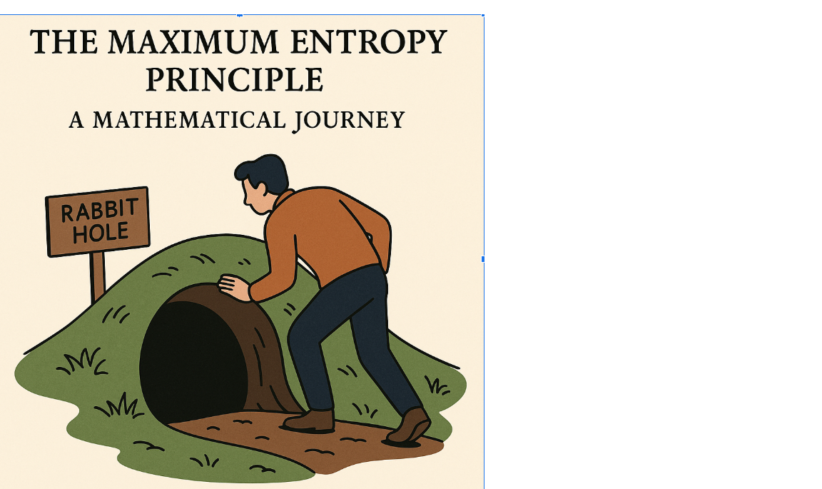
At first, I didn’t quite follow his line of thought, so I asked him to clarify. He explained: in some situations we use one distribution, in other situations another, so how do we make the right choice?

My initial reaction was to brush it off with a simple answer: “That’s just the way it is. We know this from physical cases.” But something stopped me. That kind of response is exactly the kind I dislike receiving myself: closed, dismissive, and unsatisfying.

I had to pause and ask myself: Am I becoming the narrow-minded mathematician who takes things for granted?

I realized I couldn’t give him that answer. Not just for his sake, but for my own.

A simple question led me to the Maximum Entropy Principle, a deceptively simple idea that unfolds into a rich and elegant theory. This post is the story of that discovery.

It all began with an intuition. The idea is simple: when we need to choose a probability distribution but only have partial knowledge, like an average value or a variance, the fairest choice is the one that adds no extra assumptions. In practice, that means picking the distribution with the highest entropy: the one that remains as uncertain or ‘messy’ as possible while still honoring what we know. For example, if all you know about a die is that its average roll is 3.5, the natural conclusion is that each side is equally likely. That’s the maximum entropy distribution at work.

Next, we’ll shift from intuition to mathematics and see how to express this principle in a precise, formal way.

Mathematically, the entropy of a probability distribution p(x) is defined as

H(p)=−∑xp(x)log(⁡p(x)), for discrete outcomes, or

H(p)=−∫p(x)log(⁡p(x)) dx, for continuous ones.

Now comes the key idea — the Maximum Entropy Principle. It says that whenever we know only part of the story, like a mean or a variance, the fairest choice is to pick the distribution that spreads our uncertainty as widely as possible while still honoring those facts. In other words, we don’t sneak in hidden assumptions — we let the data we do know set the rules, and keep everything else as open and unbiased as possible.

Next, let’s bring the principle down to earth with a simple example. The cleanest place to start is the uniform distribution, our most straightforward case, so we’ll begin there.

Maximum Entropy → Uniform Distribution

The Maximum Entropy Principle can be stated formally as follows: choose the probability distribution p(x) that maximizes the entropy

subject to the constraints we already know. At the most basic level, the only constraint is that p(x) must be a valid probability measure, meaning the probabilities are non-negative and sum to one.

Step 1. Constraint: probabilities must be non-negative and sum to one

We assume that all outcomes are possible, but we have no further information.

Since this is a probability measure we have the following constraints,

Step 2. Lagrangian formulation

From optimization theory, problems with constraints can be solved using the method of Lagrange multipliers. Introducing a multiplier λ\lambdaλ for the normalization constraint, the Lagrangian becomes

The stationarity condition gives

The KKT conditions further imply that

Thus, all probabilities are strictly positive and equal. I.e., p= 1/n

The Maximum Entropy Principle tells us that without any additional information, the fairest distribution is the uniform one: every outcome is equally likely.

Step 3. Reparameterization with Softmax

An alternative way to guarantee positivity is to reparameterize the probabilities using the softmax function:

This form automatically satisfies

regardless of the values of the parameters of θ.

Maximizing entropy over all of the θ leads again to the uniform distribution, since the optimal solution is achieved when all of the θ​ are equal.

Yes, I realize I changed the constraint from non-negative to strictly positive. This adjustment, however, enables the introduction of the softmax representation, which plays a central role in deep learning in particular, and in machine learning more broadly

Conclusion

The Maximum Entropy Principle tells us that without any additional information, the fairest distribution is the uniform one: every outcome is equally likely. The two approaches (i) optimization with KKT conditions and (ii) reparameterization with the softmax both lead to the same conclusion while ensuring probabilities remain positive.

After all of this math, let us see a simple real-life example.

Everyday Intuition: Rolling Dice

Imagine you are rolling a fair six-sided die, but you have no information about whether some faces are heavier, biased, or more likely to appear.

The only facts you can be sure of are:

• There are 6 possible outcomes: 1 through 6.
• The probabilities must add up to 1.

That’s exactly the setup of the Maximum Entropy Principle: no extra information, just the number of outcomes.

So the “least biased” assignment is to give each face the same probability:

p(1)=p(2)=⋯=p(6)=1/6.

Intuition:

The uniform distribution is like saying, “until I have evidence otherwise, I’ll treat all outcomes equally.” It’s the most cautious and fair way to assign probabilities, spreading uncertainty evenly, instead of favoring one side without reason.

Although the die example feels obvious, it points toward a general method: we can systematically derive probability distributions from whatever prior knowledge we have. When that knowledge is simple, the solution is straightforward, but as the constraints grow more complex, the optimization becomes less trivial. Fortunately, even the basic tools of calculus and differential equations are enough to solve these problems. To see this in action, the table below shows several classic probability distributions and the specific constraints that the Maximum Entropy Principle uses to bring them to life.

What ties these examples together is that they all belong to the exponential family of distributions. The Maximum Entropy Principle ensures that once we specify certain constraints, such as the mean, variance, or median, the resulting distribution naturally takes the exponential-family form:

where T(x) are the sufficient statistics, θ are the natural parameters, and A(θ) is the log-partition function that guarantees proper normalization.

One way to picture this is to think of the exponential family as a kind of molding machine. The constraints we impose (mean, variance, counts, and so on) are like settings on the machine. Adjusting them produces different shapes: uniform, exponential, Gaussian, or Poisson distributions.

In this sense, maximum entropy is not just a clever mathematical shortcut but a structural principle, a blueprint that quietly shapes many of the most common distributions in probability, statistics, and machine learning.

It is worth emphasizing that not every probability distribution belongs to the exponential family. A well-known counterexample is the Cauchy distribution, celebrated (and sometimes dreaded) for its heavy tails and the absence of a defined mean or variance. Because the exponential family relies on moment-based constraints, the Cauchy distribution falls outside its scope. Another important example is mixture models, such as Gaussian mixtures. These cannot be expressed with a single set of sufficient statistics and natural parameters, since their structure inherently combines multiple components. In short, while the exponential family is broad and mathematically elegant, its reach does not extend to every distribution.

At first glance, the log-partition function is just a technical detail. In fact, it sits at the very heart of the exponential family. Denoted A(θ), its primary role is to ensure the distribution is properly normalized — so that all probabilities sum (or integrate) to one. Formally,

or the corresponding integral in the continuous case.

But A(θ) is far more than a bookkeeping tool: it encodes the essential structure of the distribution itself. The gradient of A(θ) gives the expected values of the sufficient statistics, while its Hessian reveals their variances and covariances. Intuitively, you can think of the log-partition function as a control panel, set the parameters θ, and A(θ) translates those settings into concrete statistical features such as mean, variance, and correlations. This makes it a central object not only in probability theory but also in machine learning, where it governs optimization, inference, and even connects to the notion of free energy in physics.

Example: The Bernoulli distribution

For a Bernoulli random variable X∈{0,1} with parameter p, the probability mass function is

We can rewrite this in exponential-family form:

where the natural parameter is

and the log-partition function is

• Gradient:

which gives the expected value of X.

• Hessian:

which is the variance of X.

Intuition: The log-partition function A(θ) automatically encodes everything we care about: the mean, the variance, and the normalization. It’s like the “master switchboard” of the distribution.

This connection is exactly what underlies logistic regression. In logistic regression, each outcome is modeled as a Bernoulli random variable in the exponential family, with the natural parameter θ expressed as a linear function of the input features:

Through the log-partition function

The model ensures proper normalization and links the linear predictor to the probability

In other words, logistic regression isn’t just some arbitrary modeling trick; it naturally falls out of the exponential family framework for Bernoulli outcomes. The log-partition function quietly does the heavy lifting, transforming raw feature weights into proper probabilities. I wasn’t expecting this connection when I first came across it, but that’s the beauty of mathematics: it reveals hidden patterns that were always there, waiting to be discovered.

Ending notes

Since we began our journey with entropy, it feels only right to end with it as well. The log-normal distribution offers a final perspective: its link to entropy can be understood through the Legendre transform. At a high level, the log-partition function and entropy are like two sides of the same coin, mathematical duals of each other. When we move from a normal distribution on log⁡(X) to the log-normal on X, the entropy carries over, blending the Gaussian’s contribution from variance with an extra term from the mean. In this way, the log-normal reminds us that entropy is not just a formula but a structural principle, one that reveals deep geometric connections across probability.

This post is just a glimpse of a much larger story. The Maximum Entropy Principle stretches well beyond the scope of this discussion, influencing probability theory, signal processing, machine learning, and even the design of large language models. I owe special thanks to the graduate student whose simple yet profound question sparked this exploration — it’s a powerful reminder that meaningful discoveries often begin with curiosity, and that fresh perspectives can open doors we didn’t even realize were there.

Yes, I first answered the graduate student using the Maximum Entropy Principle, but can we go further? The answer is yes. The Free Energy Principle builds directly on the same foundations. While maximum entropy tells us to select the most unbiased distribution consistent with our constraints, the Free Energy Principle reframes the problem dynamically: systems maintain themselves by continuously minimizing a variational free energy functional. First introduced by Karl Friston, this principle has a strong resemblance to Hamiltonian systems in physics.

In essence, just as maximum entropy ensures the “fairest” distribution under uncertainty, the Free Energy Principle explains how living and artificial systems actively reduce the mismatch between what they predict and what they observe. It transforms a static rule about distributions into a general law of adaptation, perception, and learning.

It is only fair to say that the Free Energy Principle deserves a dedicated post of its own, something I may return to in the future.

In the end, entropy is more than a measure of uncertainty, it is the quiet architect of order within chaos. It shows us how to choose when knowledge is scarce and how to shape distributions when only fragments of truth are known. From the motion of particles to the learning of machines, from the flow of time in physics to the flow of information in language, entropy is the hidden thread binding together chance and structure. It is not merely a number, but a principle, a compass guiding us through the unknown. I hope that reading this post has been as rewarding for you as writing it has been for me. Thank you for your attention.

At certain points in this post, I’ve chosen to be a bit sloppy with the details in order to keep the flow accessible. While the subject rests on solid mathematical foundations, I believe the intention matters more than strict rigor at this stage of study. As an exercise, I encourage readers to work out the regressive version on their own. And if that feels challenging, I’ll be more than happy to help.

I would like to thank my dear friend Chen Zakaim for his insightful question, thoughtful support, and valued friendship.