Mastering SARSA: Step-by-Step Implementation in Python

A Practical Beginner-to-Intermediate Guide for Building, Training, and Evaluating SARSA Agents Using Python

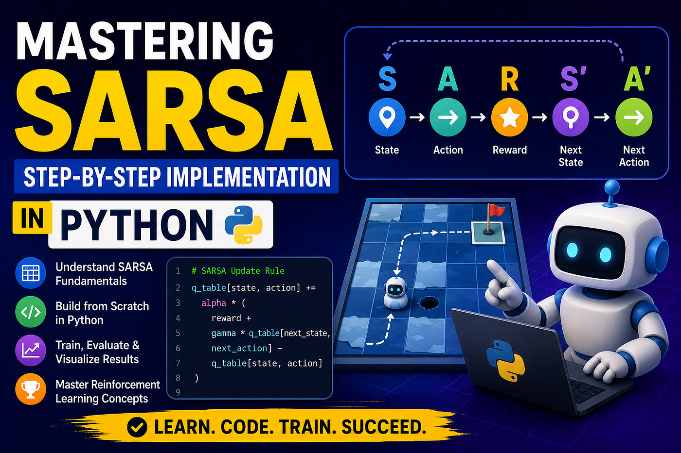
Reinforcement Learning (RL) has become one of the most exciting fields in artificial intelligence, enabling agents to learn optimal behaviors through interaction with their environment. Among the many RL algorithms available, SARSA stands out as one of the most intuitive and beginner-friendly approaches.

SARSA is an on-policy Temporal Difference (TD) learning algorithm that helps agents learn the value of actions while following a specific policy. Unlike some algorithms that learn from hypothetical best actions, SARSA learns directly from the actions it actually takes, making it more cautious and often safer in uncertain environments.

In this guide, you’ll learn what SARSA is, how it works, and how to implement it from scratch in Python using the Gymnasium library.

Understanding SARSA Fundamentals

What Does SARSA Stand For?

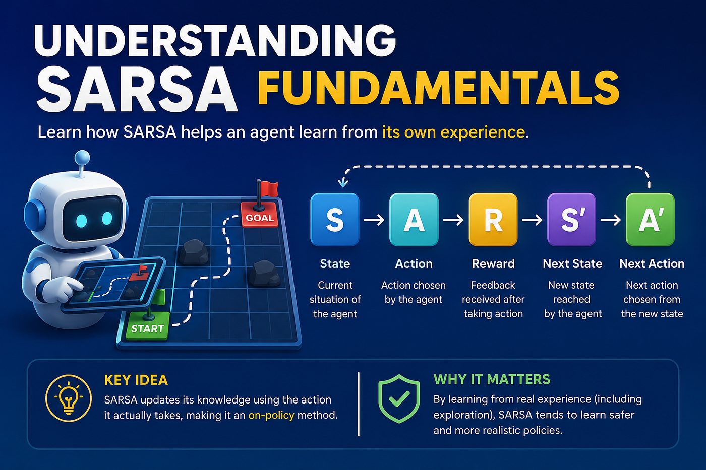
The name SARSA comes from the sequence of elements used during learning:

• State (S) — The agent’s current situation.
• Action (A) — The action chosen by the agent.
• Reward (R) — The feedback received after taking the action.
• Next State (S’) — The new state reached after the action.
• Next Action (A’) — The next action selected from the new state.

This sequence gives SARSA its name:

S → A → R → S’ → A’

Unlike Q-Learning, which updates values using the best possible future action, SARSA updates values using the action actually chosen by the current policy.

On-Policy Learning Explained

SARSA is known as an on-policy learning algorithm. This means the agent learns the value of the policy it is currently following.

Imagine you’re learning to ride a bicycle. Instead of asking what the perfect rider would do, you evaluate your own actions and improve based on your actual experiences. SARSA follows the same philosophy.

This characteristic often makes SARSA more conservative and realistic in environments containing risk.

The SARSA Algorithm

The core update equation is:

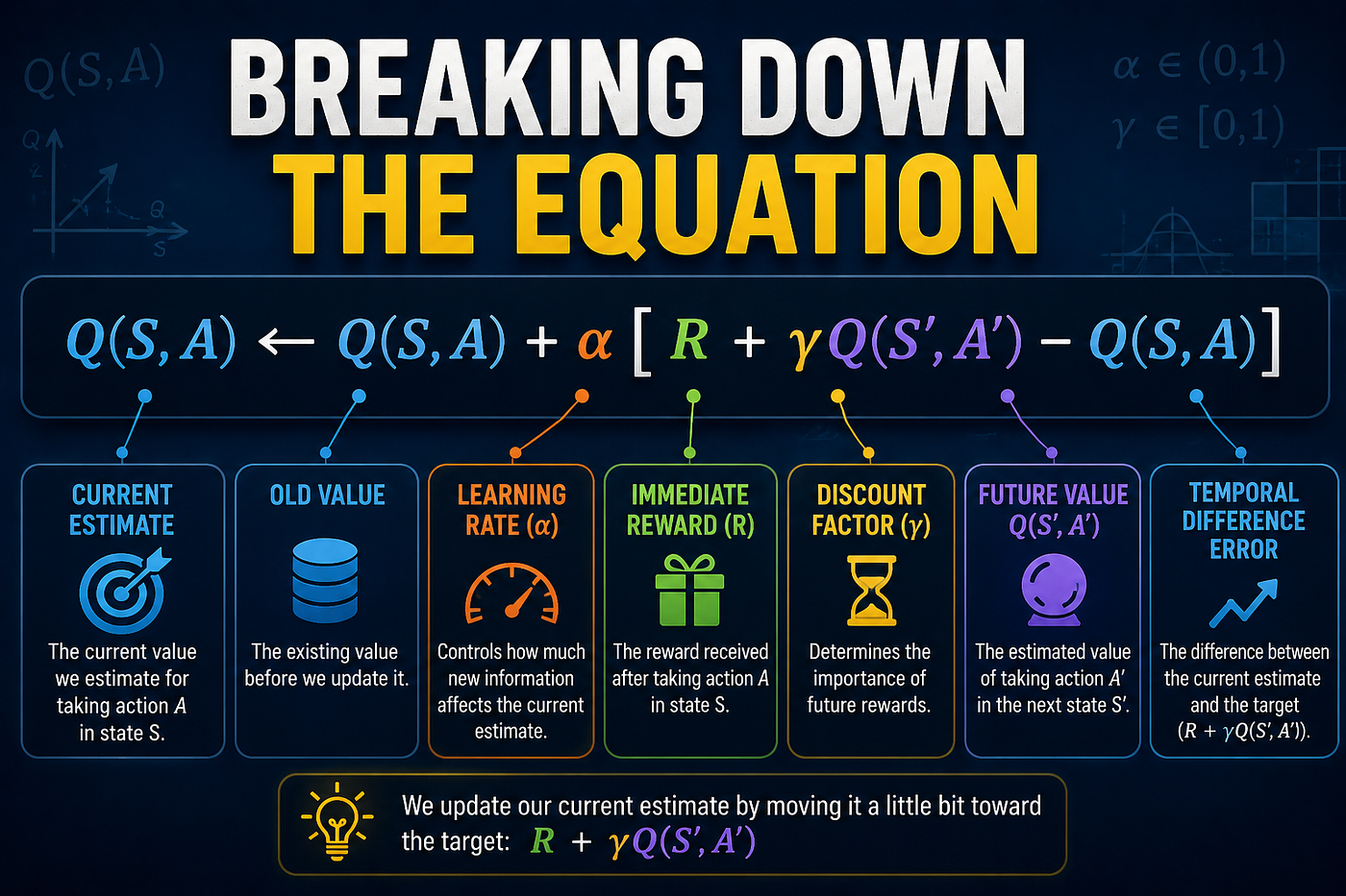
Q(S, A) ← Q(S, A) + α [R + γQ(S’, A’) − Q(S, A)]

Where:

• Q(S,A) = Current estimate
• α (alpha) = Learning rate
• R = Immediate reward
• γ (gamma) = Discount factor
• Q(S’,A’) = Future estimate

Breaking Down the Equation

Current Q-Value

Represents the current estimate of how good an action is.

Learning Rate (α)

Controls how quickly new information replaces old information.

• Small α → slower learning
• Large α → faster but potentially unstable learning

Reward (R)

The immediate feedback from the environment.

Discount Factor (γ)

Determines the importance of future rewards.

• γ = 0 focuses on immediate rewards
• γ close to 1 values long-term rewards

Temporal Difference Error

The expression:

R + γQ(S’,A’) — Q(S,A)

is called the TD Error.

It measures how wrong the current prediction is.

Setting Up the Python Environment

We’ll use the following libraries:

pip install numpy gymnasium matplotlib

Import the required packages:

import numpy as np
import gymnasium as gym
import matplotlib.pyplot as plt

Creating the Environment

For this tutorial, we’ll use FrozenLake.

env = gym.make(
    "FrozenLake-v1",
    is_slippery=False
)

Get environment dimensions:

state_size = env.observation_space.n
action_size = env.action_space.n
print(state_size)
print(action_size)

Output:

16
4

There are:

• 16 states
• 4 possible actions

Initializing the Q-Table

The Q-table stores the value of every state-action pair.

q_table = np.zeros(
    (state_size, action_size)
)

Initially, all values are zero.

Implementing ε-Greedy Action Selection

The ε-greedy strategy balances exploration and exploitation.

def choose_action(state, epsilon):
  if np.random.random() < epsilon:
    return env.action_space.sample()
  return np.argmax(q_table[state])

Why Use ε-Greedy?

Without exploration, the agent might miss better solutions. The ε parameter determines how often random actions are selected.

Implementing the SARSA Update Rule

The update rule is straightforward.

def update_q_table(
    state,
    action,
    reward,
    next_state,
    next_action
):
    q_table[state, action] += alpha * (
        reward
        + gamma * q_table[next_state, next_action]
        - q_table[state, action]
    )

This is where learning actually occurs.

Building the Training Loop

Define hyperparameters:

alpha = 0.1
gamma = 0.99

epsilon = 1.0
epsilon_min = 0.01
epsilon_decay = 0.995

episodes = 5000

Train the agent:

rewards = []

for episode in range(episodes):
    state, _ = env.reset()
    action = choose_action(
        state,
        epsilon
    )
    total_reward = 0
    done = False
    while not done:
        next_state, reward, terminated, truncated, _ = env.step(action)
        done = terminated or truncated
        next_action = choose_action(
            next_state,
            epsilon
        )
        q_table[state, action] += alpha * (
            reward
            + gamma * q_table[next_state, next_action]
            - q_table[state, action]
        )
        state = next_state
        action = next_action
        total_reward += reward
    rewards.append(total_reward)
    epsilon = max(
        epsilon_min,
        epsilon * epsilon_decay
    )

At the end of training, the Q-table contains the learned policy.

Complete SARSA Implementation

import numpy as np
import gymnasium as gym
import matplotlib.pyplot as plt

env = gym.make(
    "FrozenLake-v1",
    is_slippery=False
)
state_size = env.observation_space.n
action_size = env.action_space.n
q_table = np.zeros(
    (state_size, action_size)
)
alpha = 0.1
gamma = 0.99
epsilon = 1.0
epsilon_min = 0.01
epsilon_decay = 0.995
episodes = 5000
rewards = []
def choose_action(state, epsilon):
    if np.random.random() < epsilon:
        return env.action_space.sample()
    return np.argmax(q_table[state])
for episode in range(episodes):
    state, _ = env.reset()
    action = choose_action(
        state,
        epsilon
    )
    total_reward = 0
    done = False
    while not done:
        next_state, reward, terminated, truncated, _ = env.step(action)
        done = terminated or truncated
        next_action = choose_action(
            next_state,
            epsilon
        )
        q_table[state, action] += alpha * (
            reward
            + gamma * q_table[next_state, next_action]
            - q_table[state, action]
        )
        state = next_state
        action = next_action
        total_reward += reward
    rewards.append(total_reward)
    epsilon = max(
        epsilon_min,
        epsilon * epsilon_decay
    )
print(q_table)

Visualizing Training Performance

Plot the reward history.

plt.figure(figsize=(10,5))

window = 100
moving_avg = np.convolve(
    rewards,
    np.ones(window)/window,
    mode='valid'
)
plt.plot(moving_avg)
plt.xlabel("Episode")
plt.ylabel("Average Reward")
plt.title("SARSA Learning Curve")
plt.show()

A successful learning process typically shows increasing rewards over time.

Evaluating the Learned Policy

Disable exploration during testing.

epsilon = 0

Run several evaluation episodes.

successes = 0

for _ in range(100):
    state, _ = env.reset()
    done = False
    while not done:
        action = np.argmax(
            q_table[state]
        )
        state, reward, terminated, truncated, _ = env.step(action)
        done = terminated or truncated
    successes += reward
print(
    "Success Rate:",
    successes
)

A well-trained SARSA agent should achieve a high success rate on FrozenLake.

Hyperparameter Tuning

Learning Rate (α)

Typical values:

0.01
0.05
0.1

Higher values speed up learning but may introduce instability.

Discount Factor (γ)

Typical values:

0.90
0.95
0.99

Larger values encourage long-term planning.

Exploration Rate (ε)

A common strategy:

epsilon = epsilon * 0.995

This gradually shifts the agent from exploration to exploitation.

Advanced Improvements

Expected SARSA

Expected SARSA replaces the sampled next action with the expected value over all possible actions.

Advantages:

• Lower variance
• More stable learning
• Better convergence behavior

SARSA(λ)

SARSA(λ) introduces eligibility traces.

Benefits include:

• Faster learning
• Better credit assignment
• Improved performance in larger environments

Deep SARSA

For large state spaces, Q-tables become impractical.

Deep SARSA replaces the table with a neural network.

Applications include:

• Robotics
• Autonomous vehicles
• Strategy games
• Resource management systems

Practical Applications of SARSA

SARSA is widely used in:

Robotics

Teaching robots how to navigate safely.

Autonomous Driving

Learning driving policies under uncertainty.

Video Games

Developing adaptive AI opponents.

Industrial Automation

Optimizing manufacturing processes.

Resource Allocation

Improving scheduling and operational efficiency.

Advantages and Limitations

Advantages

• Easy to understand
• Simple to implement
• Stable learning behavior
• Considers exploration during updates
• Suitable for stochastic environments

Limitations

• Slower convergence than Q-Learning
• Requires continuous exploration
• Struggles with large state spaces
• Q-table memory requirements grow rapidly

Conclusion

SARSA remains one of the most important reinforcement learning algorithms for beginners and practitioners alike. Its on-policy nature allows it to learn directly from the actions it actually takes, often producing safer and more realistic policies than Q-Learning.

In this guide, we covered the theory behind SARSA, explored its update equation, built the algorithm from scratch, trained an agent in FrozenLake, and visualized its performance. Once you’re comfortable with SARSA, the next logical steps are to explore Expected SARSA, SARSA(λ), and Deep Reinforcement Learning methods that scale to more complex environments.

Mastering SARSA provides a solid foundation for understanding modern reinforcement learning algorithms and the principles that drive intelligent decision-making systems.