The Transformer Pipeline: A Complete Mathematical and Visual Guide

Demystifying Queries, Keys, Values, and the KV Cache — from raw text to high-dimensional tensor math.

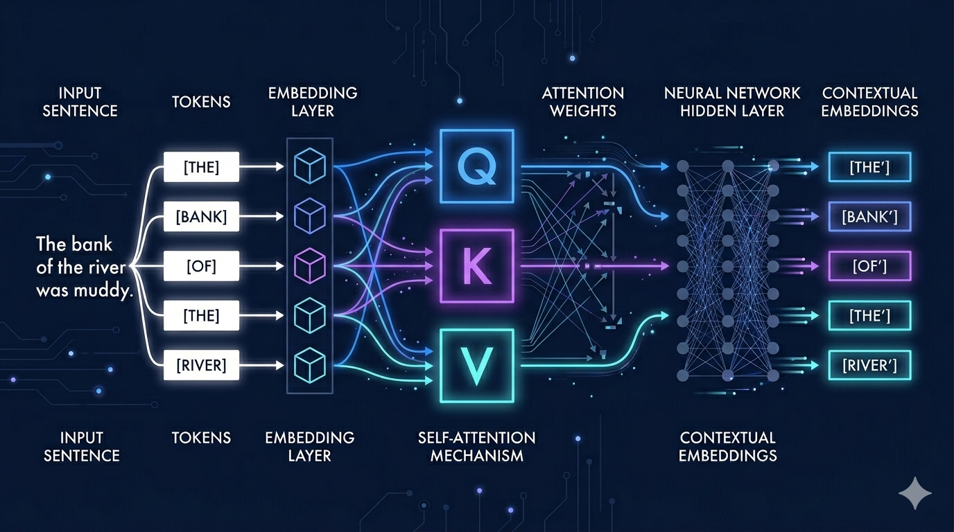
If you’ve ever felt like you’re hitting a wall trying to understand how Large Language Models (LLMs) actually work, you aren’t alone. Terms like Multi-Head Attention and KV Cache are often buried under layers of dense, academic jargon that obscure the simple, elegant math underneath.

Stop guessing how the “black box” thinks.

In this guide, we strip away the noise.

By tracking a single sentence through the entire transformer pipeline,

*Tokens → Token IDs → Embedding Vectors (X) → Multiplication by Weights (W) → Q, K, V Matrices,*

we will demystify the exact mechanics from raw text to high-dimensional tensor math.

Whether you are a developer looking to optimize inference or a student trying to bridge the gap between intuition and code, this is the deep dive you’ve been looking for.

Part 1: The Intuition Behind Q, K, and V

To understand how an LLM processes text, consider a simple search analogy. Imagine you are looking up a video on YouTube:

• The Query (Q): This is the search text you type into the search bar.
• The Keys (K): These are the video titles, descriptions, and tags in YouTube’s database.
• The Values (V): This is the actual video content you click on and watch.

In an LLM, every single token (word or sub-word) creates its own unique Query, Key, and Value vector using its own internal learned weights.

A Concrete Sentence Example

Consider this sentence:

“The bank of the river was muddy.”

How does the model figure out the exact meaning of the word “bank” (which could mean a financial institution or a slope of land)?

1. The Query (Q) asks a question: The word “bank” acts as the Query. It signals to the rest of the sentence: “I am the word ‘bank’. I need context to know what kind of bank I am. Who has clues for me?”
2. The Keys (K) offer descriptions: Every word in the sentence presents a Key vector describing what information it contains. The word “river” says: “I contain information about water, nature, and geography.” The word “muddy” says: “I contain information about wet dirt and earth.”
3. The Matchmaking Process ( Q × Kᵀ ): The model multiplies the Query vector of “bank” with the Key vectors of all other words. The math yields a massive similarity score for “river” and “muddy”, while yielding a very low score for structural words like “The”.
4. Extracting the Value (V): Because “river” and “muddy” achieved the highest attention scores, the model extracts a high percentage of their Value vectors (their actual semantic meaning) and blends them directly into the representation of “bank”.

The Result: The representation of “bank” updates dynamically from an ambiguous word into a specific concept: a slope of land next to a body of water.

Part 2: The Math of Single-Head Attention

Let’s ground this intuition into a concrete mathematical walkthrough using the standard Transformer attention formula:

To keep the matrices easy to read, let’s use a simplified 3-word phrase: “bank river muddy” with an embedding dimension (nₑ) of 2 and an attention head dimension (dₖ) of 2.

Step 0: The Projection Phase (From Embeddings to Q, K, V)

Before calculating attention, the raw text must be transformed into numbers via this pipeline:

Text → Token IDs → Embedding Matrix (X) → Linear Projection (W) → Q, K, V

The model executes three sequential steps:

1. Tokenization: The text is split into tokens, and each token is mapped to a unique integer ID.
2. Embedding: Each token ID pulls a dense continuous vector from the model’s embedding lookup table. For our 3 tokens, this forms our raw input matrix X of shape (3, 2).
3. Linear Projection: To get Q, K, and V, we multiply X by three independent, trained weight matrices: W_Q, W_K, and W_V (each of shape (2, 2)).

Let’s have a look how the Query Matrix (Q) is born. Imagine our raw token embedding matrix X looks like this:

To project these embeddings into the Query space, we multiply X by the model’s learned Query weights (W_Q):

For the single token “bank” (represented by the vector [1.00, 0.50]), the matrix multiplication works row-by-column:

Repeating this matrix multiplication (X × W_Q) for all rows yields our complete Q matrix. The exact same operation is performed with W_K and W_V to generate the K and V matrices.

Step 1: Examine the Final Projected Matrices (Q and K)

Query Matrix (Q) — What each word wants

Key Matrix (K) — What each word offers

Step 2: Calculate Raw Similarity Scores (Q × Kᵀ)

We multiply every row of Q by every transposed row of K (dot product) to find their raw alignment scores. For example, for the token pair (bank × muddy), the calculation is:

(−0.46 × −0.47) + (0.94 × 0.65) = 0.83

Raw Scores Matrix:

Step 3: Scale Down (÷ √dₖ)

If our vectors are long, dot products yield large values that push the Softmax function into regions with near-zero gradients, stalling model training. To stabilize this, we divide our scores by the square root of our key dimension (√dₖ = √2 ≈ 1.41).

Scaled Scores Matrix:

Step 4: Convert to Percentages (Softmax)

Applying Softmax row-by-row turns these values into positive fractions that sum up to exactly 1.00 (100%).

Softmax Attention Matrix:

The Blueprint: Look at the first row (bank). The model mathematically decides to assign 49% of its attention to “muddy”, 20% to “river”, and 31% to itself. These percentages multiply directly with the Value matrix (V) to create the final, blended contextual representation.

Part 3: Scaling to Multi-Head Attention and 4D Tensors

In production, models don’t rely on a single attention head. They use Multi-Head Attention (MHA) to look for multiple distinct semantic relationships at the same time.

Crucially, heads do not slice up the word into separate parts. Every head evaluates the entire text, but each head uses a unique set of trained weight matrices (W_Q, W_K, W_V).

Think of it like placing multiple specialized cameras around a statue: one camera captures structural details (grammar), another captures surface texture (sentiment), and a third captures physical proximity (contextual meaning).

Let’s track exactly how the mathematical tensor shapes scale when handling real production configurations:

• Batch Size (B) = 2 (Processing two sentences concurrently)
• Context Length (N) = 5 tokens per sentence
• Embedding Dimension (nₑ) = 384
• Number of Attention Heads (H) = 6

The Head Dimension Math

The total embedding dimension is evenly divided among the attention heads:

Tracking the Tensor Shapes

1. The Input Tensor (X): Shape is (2, 5, 384) → (Batch, Tokens, Embedding_Dim).
2. The Fused Projections: Rather than looping through 6 heads sequentially, GPUs pack the weights into a single giant (384, 384) matrix. Multiplying the input tensor by this weight matrix yields a projection tensor of shape (2, 5, 384).
3. Reshaping to 4D: To keep head calculations independent, the GPU reshapes and transposes this matrix into a standard 4D layout: (2, 6, 5, 64) → (Batch, Heads, Tokens, Head_Dim)
4. 4D Attention Scoring (Q × Kᵀ): The GPU performs a Batch Matrix Multiplication exclusively on the last two axes (5, 64) × (64, 5), resulting in an attention score weight tensor of shape (2, 6, 5, 5). Each batch and head receives its own dedicated (5, 5 ) attention grid!

Part 4: The Ultimate Bottleneck Savior — The KV Cache

When an LLM generates text, it acts as an autoregressive loop (generating text token by token).

Generation Without a KV Cache (The O(n²) Nightmare)

When Token #6 arrives in the system, a model without a KV cache must re-process all 5 previous tokens alongside it. It must re-run the entire pipeline from scratch, recalculating the Key and Value matrices for old tokens repeatedly. As context windows grow to thousands of tokens, this computational overhead scales quadratically, severely slowing down generation speed.

Generation With a KV Cache (The Linear O(n) Solution)

The KV Cache bypasses this redundant work by locking the computed Key (K) and Value (V) states of past tokens directly inside the GPU’s memory. When Token #6 arrives, the model transitions from the Prefill Phase to the Decoding Phase.

Here is how the 4D tensor math morphs to optimize this step:

• Single Token Input: The model receives only the brand-new 6th token. Its input tensor shape drops down to (2, 1, 384) (only 1 token instead of 5).
• Linear Projections: Projecting this single token gives a new Query, Key, and Value tensor, each shaped as (2, 6, 1, 64).
• The Cache Update: The system pulls the past cache tensor (2, 6, 5, 64) from memory and concatenates the new token states directly along the token axis:

Cache (2, 6, 5, 64) + New Token (2, 6, 1, 64) → (2, 6, 6, 64)

• Attention Calculation (Q₍new₎ × K₍cached₎ᵀ): The isolated Query tensor of Token #6 multiplies against the fully accumulated Key cache:

(2, 6, 1, 64) × (2, 6, 64, 6) → (2, 6, 1, 6)

The final attention matrix drops to a lean shape of (2, 6, 1, 6). Instead of running heavy square matrix math, Token #6 merely computes a single row of 6 percentage values showing how much it relates to the historical context.

By keeping past token computations frozen in memory, the model reduces processing complexity down to a linear scale, maintaining rapid response times even over massive context windows.

Conclusion

Understanding Transformers doesn’t require staring blindly at abstract equations. At its core, the attention mechanism relies on basic vector matching — reshaped and packed into highly efficient 4D tensors so GPUs can compute them in parallel. By combining specialized Multi-Head weights with memory-saving KV Caching, LLMs achieve the ideal balance between deep contextual comprehension and blistering inference speeds.

References & Further Reading

To learn more about the formal frameworks, engineering structures, and mathematical proofs mentioned throughout this article, explore the authoritative research papers below:

• [1] Vaswani, A., Shazeer, N., Parmar, N., Uszkoreit, J., Jones, L., Gomez, A. N., Kaiser, Ł., & Polosukhin, I. (2017). Attention Is All You Need. Advances in Neural Information Processing Systems (NeurIPS), 30, 5998–6008. (The foundational paper that introduced the Transformer architecture, Multi-Head Attention, and the QKV framework).
• [2] Kwon, W., Li, Z., Zhuang, S., Sheng, Y., Zheng, L., Yu, C., Gonzalez, J. E., Zhang, H., & Stoica, I. (2023). Efficient Memory Management for Large Language Model Serving with PagedAttention. Proceedings of the 29th Symposium on Operating Systems Principles (SOSP), 611–626. (The baseline paper for modern KV Cache architectures, virtual memory paging blocks, and high-throughput serving systems).