How Optimizers Behave Under Noisy Labels

Introduction

This article will explore the experiment I performed while playing around with optimizers. Specifically this experiment used Adam and SGD. Earlier I used to thought SGD was some relic of past now rendered useless by more advanced optimizers. Needless to say I was very wrong. I have been recently doing some digging and discovered lot of interesting literature about Adaptive and Non-Adaptive optimizing techniques that I will be sharing in future articles.

“This experiment does not aim to rank optimizers universally, but to expose how optimizer choice interacts with noisy supervision. Label noise here acts as a proxy for spurious features. the goal is mechanistic insight, not state-of-the-art performance.”

Setup

I trained 2 instances of a small CNN model on subset of MNIST dataset using SGD and Adam. I injected dirty labels to 20% of the training data to see how optimizers react to it (since no one is perfect and optimizers should keep it in mind). Adam overfit immediately, reaching Training accuracy of 100% even memorizing the spurious datapoints. SGD resists overfitting and thus performs more robustly. Also the Adam-Trained model was more sensitive to small perturbation while SGD-Trained model showing more robustness to small perturbations. From the sensitivity analysis, one can deduce that Adam-Trained model converged into a sharp minima while SGD-Trained one converged to relatively flatter region.

Misconception

“Optimizers only affect how fast a model trains, not which solution it ultimately converges to.”

When training data contains spurious or noisy signals, different optimizers converge to different solutions with different generalization behavior, even when architecture and data are fixed.

Growing model complexity usually leads to loss of convexity of loss curves and we get many minima regions and choice of optimizer can nudge the model in direction of different solutions.

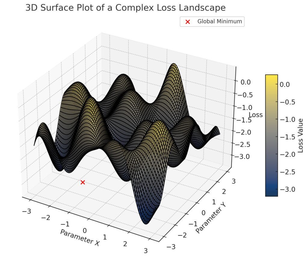
Hot and Curvy Loss Landscape

Preparing Dataset

Here I took only 10% of original dataset because I lack patience of training the model on whole 60K datapoints and for our purposes this reduced dataset will be enough.

import torch, torchvision
from torchvision import datasets, transforms
import numpy as np
import pandas as pd
import matplotlib.pyplot as plt
from torch import nn
from torch.utils.data import Subset

train_data = datasets.MNIST(
    root='data',
    train=True,
    download=True,
    transform=transforms.ToTensor(),
    target_transform=None
)
test_data = datasets.MNIST(
    root='data',
    train=False,
    download=True,
    transform=transforms.ToTensor(),
    target_transform=None)

print("Training set size:", len(train_data))
print("Test set size:", len(test_data))

# creating subset only 10% of whole
torch.manual_seed(42)

random_indices = torch.randperm(train_data.__len__()-1).tolist()[:6000]
reduced_train_data = Subset(train_data, random_indices)
random_indices = torch.randperm(test_data.__len__()-1).tolist()[:1000]
reduced_test_data = Subset(test_data, random_indices)

Adding Noise to the Data

Flipped the labels of 20% datapoints. Here I tried to keep the nomenclature of methods consistent with Pytorch’s official dataset method names. Hence, the names len and getitem. (Consistency makes code Pretty)

Spurious data exposes optimizer bias

from torch.utils.data import Dataset, DataLoader

class NoisyLabelsDataset(Dataset):
    def __init__(self, base_dataset, noise_ratio=0.2, num_classes=10, seed=42):
        self.base_dataset = base_dataset
        self.noise_ratio = noise_ratio
        self.num_classes = num_classes

        g = torch.Generator().manual_seed(seed)

        self.noisy_indices = torch.rand(len(base_dataset), generator=g) < noise_ratio
        self.random_labels = torch.randint(
            0, num_classes, (len(base_dataset),), generator=g
        )

    def __len__(self):
        return len(self.base_dataset)

    def __getitem__(self, idx):
        x, y = self.base_dataset[idx]

        if self.noisy_indices[idx]:
            y = self.random_labels[idx]
        y = torch.tensor(y, dtype=torch.long)
        return x, y

noisy_train_dataset = NoisyLabelsDataset(
    reduced_train_data,
    noise_ratio=0.2
)
train_dataloader = DataLoader(
    noisy_train_dataset,
    batch_size=64,
    shuffle=True
)
test_dataloader = DataLoader(reduced_test_data, batch_size=64, shuffle=True)

Model Architecture

class classifier_model(nn.Module):
  def __init__(self):
    super().__init__()
    self.covnet = nn.Sequential(
        nn.Conv2d(in_channels = 1, out_channels=32, kernel_size=3, padding=1),
        nn.ReLU(),
        nn.Conv2d(in_channels = 32, out_channels=64, kernel_size=3, padding=1),
        nn.ReLU(),
        nn.Flatten(),
        nn.Linear(in_features = 50176, out_features=3136),
        nn.ReLU(),
        nn.Linear(in_features = 3136, out_features = 256),
        nn.ReLU(),
        nn.Linear(in_features = 256, out_features = 10)
    )
  def forward(self, x):
    z = self.covnet(x)
    return z

Training Loop

Learning rates for SGD and Adam are different in the code. This decision is merely consequence of the fact that SGD converges slower than Adam. You can reduce the learning rate of SGD to make it same as Adam’s but Then you will have to increase the epochs for sgd_model training and give it time to converge.

from tqdm import tqdm

def train_model(
    model,
    train_dataloader,
    test_dataloader,
    optimizer,
    loss_fn,
    epochs=10,
    device='cuda' if torch.cuda.is_available() else 'cpu'
):
  model.to(device)
  train_acc_history = []
  val_acc_history = []

  for epoch in tqdm(range(epochs)):
    model.train()
    train_loss = 0.0
    train_correct = 0
    train_total = 0

    for x, y in train_dataloader:
      x = x.to(device)
      y = y.to(device)

      logits = model(x)
      loss = loss_fn(logits, y)

      optimizer.zero_grad()
      loss.backward()

      optimizer.step()

      train_loss += loss.item() * x.size(0)
      preds = torch.argmax(logits, dim=1)
      train_correct += (preds == y).sum().item()
      train_total += x.size(0)

    train_loss /= train_total
    train_acc = train_correct / train_total
    train_acc_history.append(train_acc)

    model.eval()

    val_loss = 0.0
    val_correct = 0
    val_total = 0
    with torch.inference_mode():
      for x, y in test_dataloader:
        x = x.to(device)
        y = y.to(device)

        logits = model(x)
        loss = loss_fn(logits, y)
        val_loss += loss.item() * x.size(0)
        preds = torch.argmax(logits, dim=1)
        val_correct += (preds==y).sum().item()
        val_total += x.size(0)

    val_loss /= val_total
    val_acc = val_correct / val_total
    val_acc_history.append(val_acc)

    print(
      f"Epoch [{epoch+1}/{epochs}] | "
      f"Train Loss: {train_loss:.4f}, Train Acc: {train_acc:.4f} | "
      f"Val Loss: {val_loss:.4f}, Val Acc: {val_acc:.4f}"
    )
  return train_acc_history, val_acc_history

epochs_adam = 50
epochs_sgd = 50
device = "cuda" if torch.cuda.is_available() else "cpu"
loss_fn = nn.CrossEntropyLoss()

# SGD
model_sgd = classifier_model()
optimizer_sgd = torch.optim.SGD(
    model_sgd.parameters(),
    lr=0.006,

)

sgd_train_acc, sgd_val_acc = train_model(
    model_sgd,
    train_dataloader,
    test_dataloader,
    optimizer_sgd,
    loss_fn,
    epochs_sgd,
    device
)

# Adam
model_adam = classifier_model()
optimizer_adam = torch.optim.Adam(
    model_adam.parameters(),
    lr=1e-3,
)

adam_train_acc, adam_val_acc = train_model(
    model_adam,
    train_dataloader,
    test_dataloader,
    optimizer_adam,
    loss_fn,
    epochs_adam,
    device
)

Comparison: Accuracy Plot

Adam (green dashed, red solid) rapidly drives the training accuracy to nearly 100%, indicating that it successfully fits the training data, including corrupted labels. However, this aggressive fitting does not translate to better generalization. After an initial rise, Adam’s validation accuracy peaks early and then stagnates or slightly degrades, stabilizing well below its training performance.

In contrast, SGD (blue dashed, orange solid) learns more slowly and never reaches perfect training accuracy. Importantly, its validation accuracy continues to improve over time and ultimately exceeds Adam’s validation performance, despite SGD having significantly lower training accuracy throughout. SGD’s slower, noisier updates act as an implicit regularizer that limits memorization and favors more robust features.

“The plot therefore illustrates that, under noisy supervision, optimizer choice influences not just convergence speed, but the nature of the solution itself.”

import matplotlib.pyplot as plt

epochs_range_adam = range(1, epochs_adam + 1)
epochs_range_sgd = range(1, epochs_sgd + 1)

plt.figure(figsize=(8, 6))

# SGD
plt.plot(epochs_range_sgd, sgd_train_acc, label="SGD Train", linestyle="--")
plt.plot(epochs_range_sgd, sgd_val_acc, label="SGD Val")

# Adam
plt.plot(epochs_range_adam, adam_train_acc, label="Adam Train", linestyle="--")
plt.plot(epochs_range_adam, adam_val_acc, label="Adam Val")

plt.xlabel("Epoch")
plt.ylabel("Accuracy")
plt.title("SGD vs Adam: Train vs Validation Accuracy")
plt.legend()
plt.grid(True)
plt.show()

A note on early stopping

One might argue that Adam’s early validation peak suggests that an early-stopped Adam model could outperform SGD. This is a valid observation. However, early stopping itself acts as an explicit regularization mechanism, preventing the optimizer from continuing to fit spurious labels.

From this perspective, the comparison highlights a deeper difference. SGD exhibits an implicit resistance to memorization, continuing to improve validation performance without requiring careful stopping criteria, while Adam relies more heavily on explicit regularization choices to avoid overfitting noisy supervision.

In other words, the result is not that Adam cannot generalize, but that the optimizer’s default dynamics matter when regularization is not carefully tuned.

Sensitivity

To probe the local geometry of the final solutions, I measured how sensitive the loss is to small random perturbations of the parameters.

ΔL(ϵ) = L(w+ϵ⋅δ) − L(w)

For increasing perturbation magnitudes ε, the loss around the Adam solution rises more rapidly than around the SGD solution. This suggests that Adam converges to regions of the loss landscape that are more sensitive to parameter perturbations, while SGD favors flatter regions.

import copy

x_probe, y_probe = next(iter(test_dataloader))
x_probe = x_probe.to(device)
y_probe = y_probe.to(device)  

def loss_vs_perturbation(
    model, 
    loss_fn, 
    x, 
    y, 
    epsilons, 
    trials = 5
  ):
  base_loss = loss_fn(model(x), y).item()
  deltas = []

  for eps in epsilons:
    max_delta = 0.0

    for _ in range(trials):
      model_copy = copy.deepcopy(model)
      with torch.no_grad():
        for p in model_copy.parameters():
          noise = torch.randn_like(p)
          noise = eps * noise / (torch.linalg.norm(noise) + 1e-12)
          p.add_(noise)

      new_loss = loss_fn(model_copy(x), y).item()
      max_delta = max(max_delta, new_loss - base_loss)
    deltas.append(max_delta)
  return deltas

epsilons = np.logspace(-5, -1, 10)

sgd_deltas = loss_vs_perturbation(
    model_sgd, 
    loss_fn, 
    x_probe, 
    y_probe, 
    epsilons
  )
adam_deltas = loss_vs_perturbation(
    model_adam, 
    loss_fn, 
    x_probe, 
    y_probe, 
    epsilons
  )

plt.figure(figsize=(7,5))
plt.plot(epsilons, sgd_deltas, label="SGD", marker="o")
plt.plot(epsilons, adam_deltas, label = 'Adam', marker="o")
plt.xscale("log")
plt.xlabel("perturbation scale: epsilon")
plt.ylabel("Increase in loss: delta Loss")
plt.title("Sharpness comparison via parameter perturbation")
plt.legend()
plt.grid(True)
plt.show()

Conclusion

The takeaway is not that Adam fails to generalize, but that optimizer choice meaningfully shapes which solution is learned in the presence of spurious signals. When supervision is imperfect, understanding this interaction becomes as important as model architecture or dataset size. Rather than treating optimizers as interchangeable tools for speeding up training, it is more accurate to view them as implicit regularizers that influence the final model itself.