Extracting Building Data from Segmented Lidar Data

The content here was developed during the publication : Coordinated Licenced DSA for Streamlined LAL and SAL Access and Coexistence https://ieeexplore.ieee.org/document/11115929

Extracting Building Data from Segmented Lidar Data

It came to my attention that there’s no source in any platform which provides a concise way of using Lidar point cloud data to create an OSM file, using open source tools such as QGIS and JOSM, while this may be possible with ArcGIS Pro etc.

In this blog, I present a procedure to extract the building Lidar data in .Laz format to OSM format, which could be processed using many software tools, using QGIS open source geographical information software tool. We will convert this to the OSM format. I’m using the Lidar data collected by Defra, and segmented using their automated classification process, based ASPRS LAZ 1.4 standard (Ground = 2, High vegetation = 5, Buildings = 6 etc.).

Load the Lidar point cloud data to QGIS.

From version 3.18 onwards, QGIS supports loading .laz files. Using Layer > Data Source manager > Point Cloud, locate your .laz file and load it to the QGIS by clicking on “Add”. If you have multiple lidar datasets you have to use to generate the scenario from, load all the point clouds and use Point Cloud Data Management > Merge, to select all the layers and merge (Deselect and remove original lidar layers once merged layer is created).

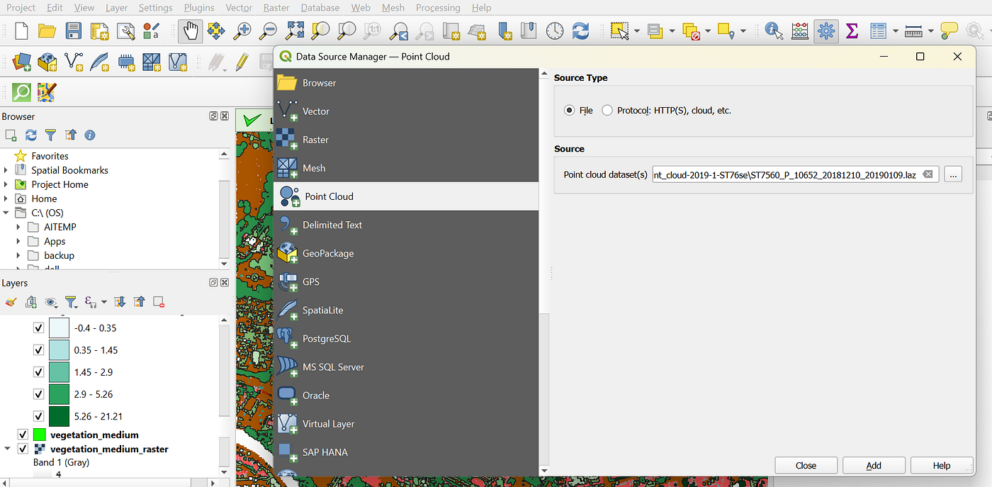
Point cloud loading.

Extract the DTM.

First we prepare a Digital Terrain Model (DTM) using lidar data, which is an elevation model of the bare earth. With the loaded lidar dataset, having this lidar data layer selected, navigate to Point Cloud Conversion > Export to Raster. A raster layer is a 2D projection image of the 3D point cloud to the ground layer, with intensity value being the elevation. In the dialogue box that appears, use attribute as Z, which corresponds to height, and filter expression Classification = 2, which corresponds to lidar data with the classification ground. Use a cropping extent if you only focus on a small area.

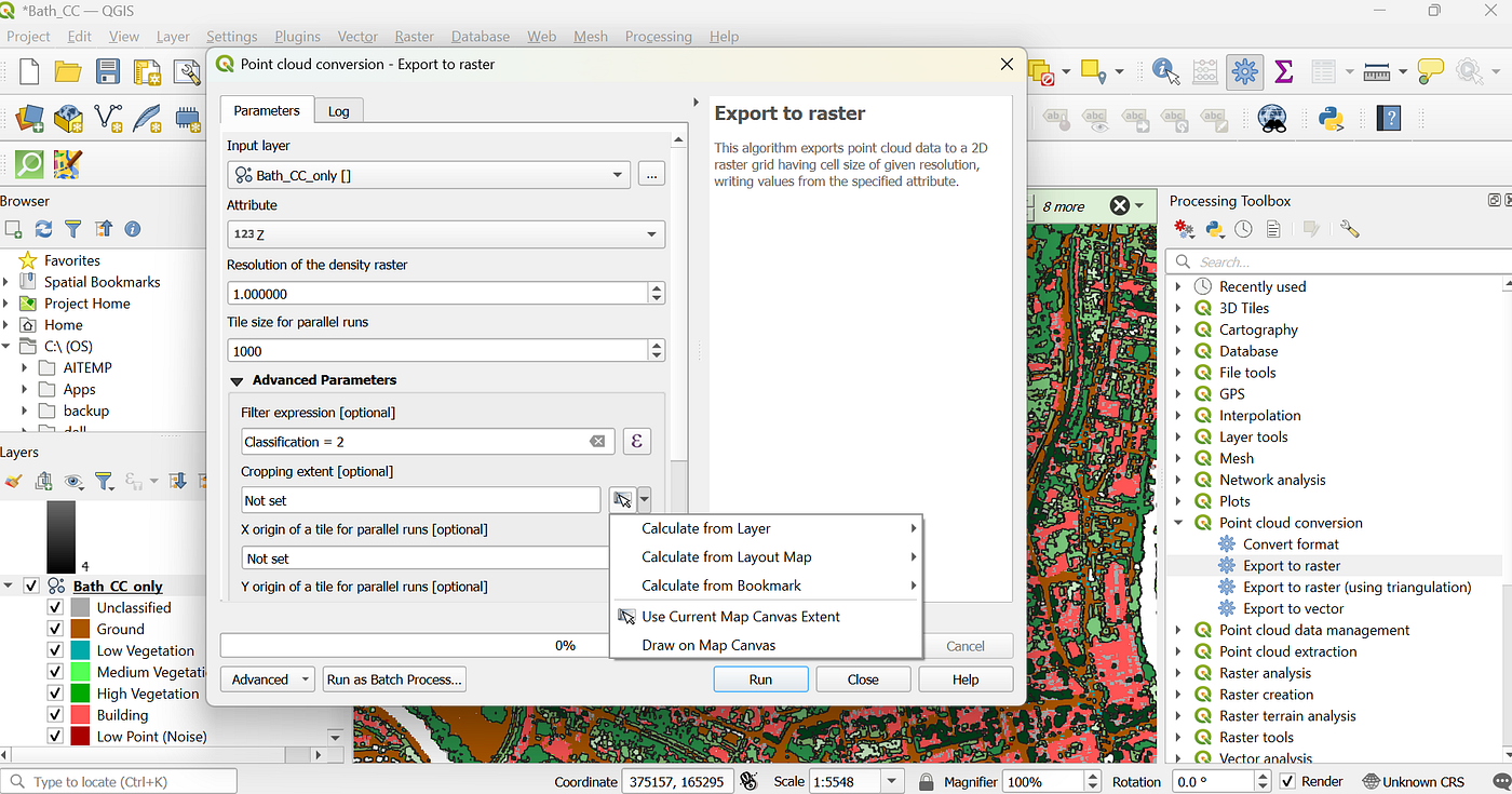
Preparation of DSM unpreprocessed Raster layer.

Once you run the conversion, the Raster layer will be appeared, but you will observe that some unfilled areas are there in the raster, which corresponds to the areas with buildings, vegetation etc.

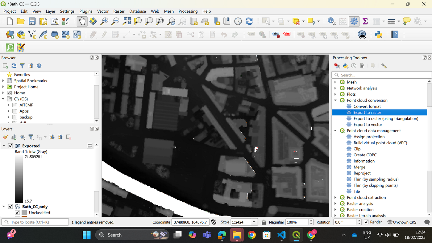
Un-preprocessed Raster layer

Use the Raster analysis > Fill NoData tool to fill the area ( Select the previously expoted layer as the input in the dialogue box) by selecting an appropriate interpolation pixel level.

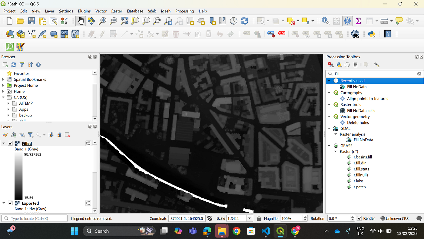
Filled Raster layer

Now rename this layer to “DTM”, because this is going to be our DTM.

Extract the DSM.

Next we need to extract a Digital Surface Model, which is the variation of the height of earth surface with all the man made (Buildings) and natural elements (vegetation).

Follow the same steps for the DTM Layer preparation, but for the creation of the the initial raster layer from the point cloud, use the evalutation expression Classification != 7 which discards Low Point (Noise) during the layer preparation. The final no data filled layer is the DSM.

Extract the height layer.

With DSM and DTM in hand, we can now calculate the variation of height in man made as well as natural entities on the earth surface.

Use Raster > Raster Calculator from the top panel, and Subtract the DTM from DSM. Save the output which is a good practice as you store these temporary intermediate layers.

Raster Calculator to calculate heights.

The resulting layer is your height layer. Rename it accordingly.

Extract building footprints

Step 1 : Prepare the building Raster layer.

Having the point cloud selected, navigate to Point Cloud Conversion > Export to Raster and use attribute “classification” to prepare the building raster layer. Use the filter expression classification = 2 and Run.

Step 2 : Extract the footprint vectors.

We need to extract the buildings out of this raster layer now. Navigate to Raster > Conversion > Polygonize ( Raster to Vector), which provides you with the building footprint polygons.

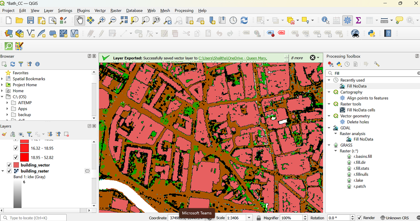
Building polygon vector layer, on top of lidar data.

Calculate the building heights.

Next we use the prepared building footprints vectors and the height layer to calculate the building heights. Use Raster analysis > Zonal Statistics to calculate the statistics such as mean, max, min height within building footprint polygons. Use Building vector layer as the input layer and use the height raster as the raster layer. Use zonal stats such as the Mean, Minimum and Maximum with an appriate prefix.

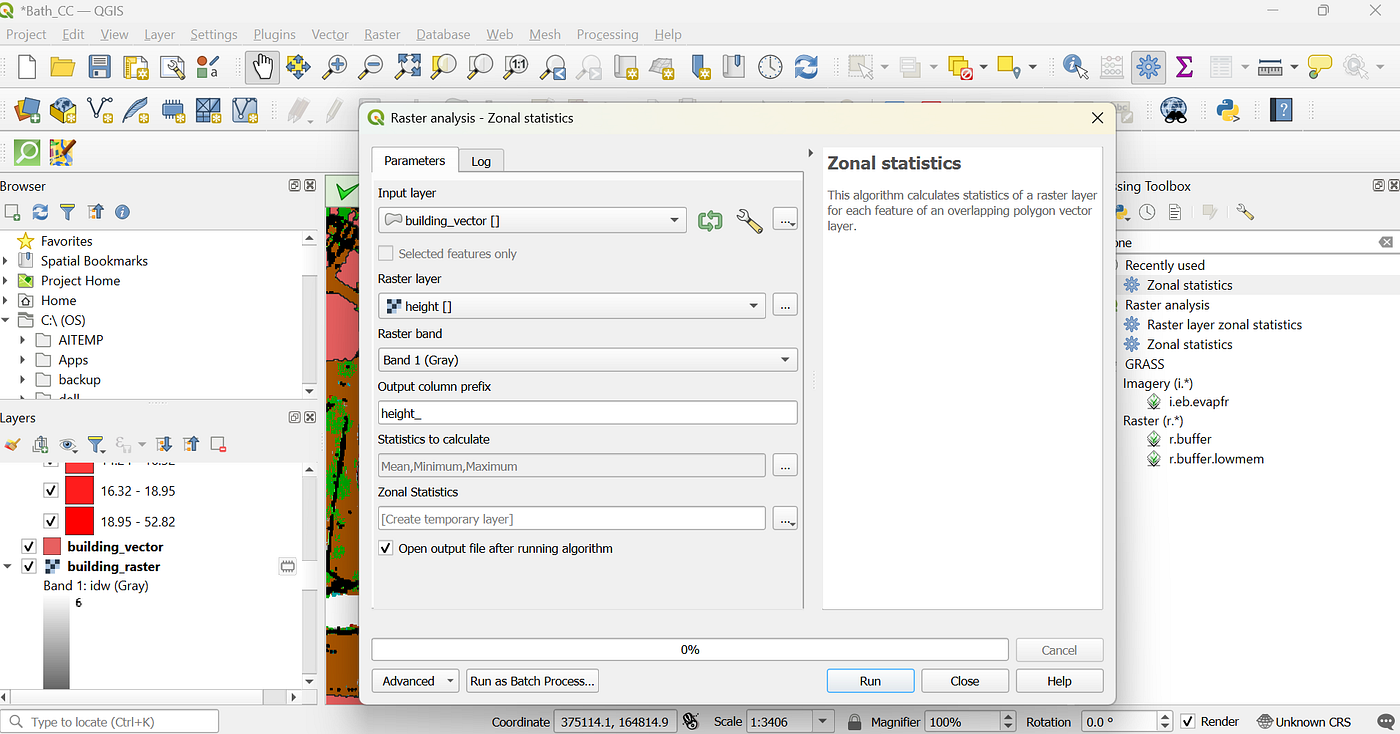
Zonal Statistics calculation.

Now you will be able to see these stats, per polygon by selecting the zonal statistics output layer > Open Attribute table. You can nicely display the buildings by height by selecting the statistics layer > properties and selecting settings appropriately like below.

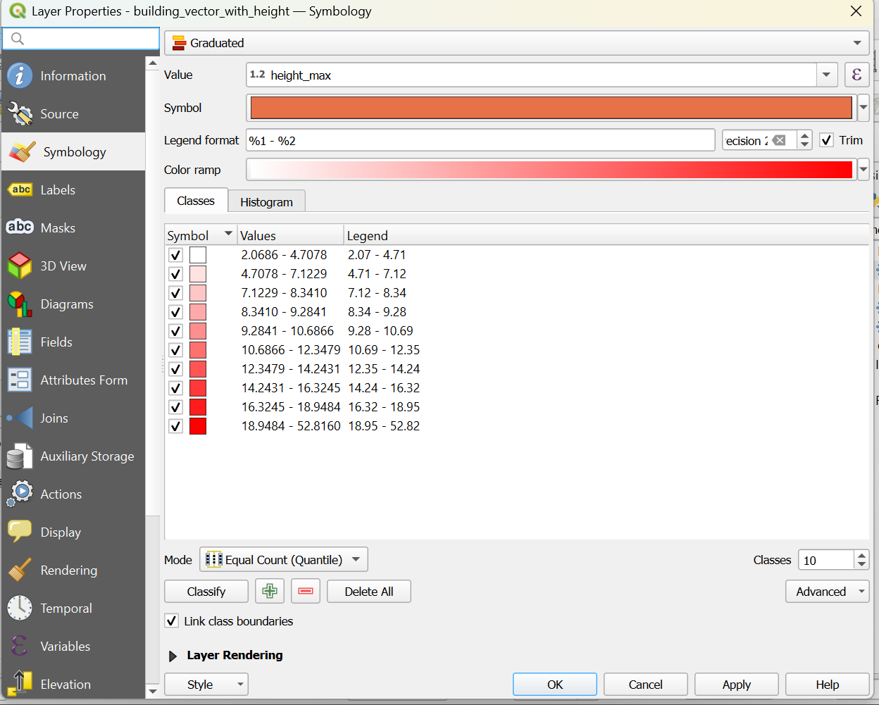
Layer properties for nice visualization.

In my file, the heights vary between 2–52 meters as it was an urban area.

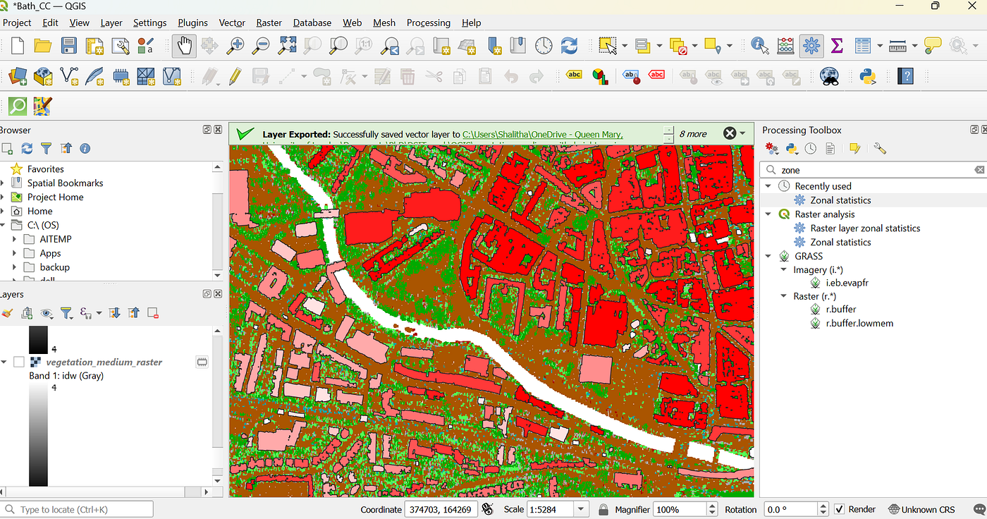
Building heights variation.

Now, export this layer via layer > Export > Save features as, to a GeoJSON file. Convert the cordinate system to WGS84 using the opened dialog box, as the OSM uses the particular CRS. The GeoJSON will have entries such as below.

{ "type": "Feature", "properties": { "fid": 4, "building": 6, "height_mean": 2.3574510574340821, "height_median": 2.4587507247924805, "height_min": 0.67704963684082031, "height_max": 3.1722621917724609 }, "geometry": { "type": "Polygon", "coordinates": [ [ [ -2.357234409339601, 51.388567001818402 ], [ -2.357234269031526, 51.388549018825763 ], [ -2.357219897961243, 51.388549062759665 ], [ -2.357219757658772, 51.388531079767006 ], [ -2.357119160204042, 51.388531387255298 ], [ -2.357119440732646, 51.388567353239914 ], [ -2.357234409339601, 51.388567001818402 ] ] ] } },

Now we have wrapped up the part we need to do using the QGIS.

Converting GEOJSON to OSM.

Next, we convert the GEOJSON to an OSM file via JOSM. Download JOSM, Load the file, and then save the file as .OSM using JOSM which is very straight forward.

Standardization of OSM

However you will see that, the OSM data in the file created using JOSM is not properly formatted as per the standard OSM data.

<relation id='-80'>
    <member type='way' ref='-700' role='outer' />
    <member type='way' ref='-701' role='inner' />
    <member type='way' ref='-702' role='inner' />
    <tag k='building' v='6' />
    <tag k='fid' v='66' />
    <tag k='height_max' v='16.218669891357422' />
    <tag k='height_mean' v='11.624085489908854' />
    <tag k='height_median' v='13.911891937255859' />
    <tag k='height_min' v='0.02512359619140625' />
    <tag k='type' v='multipolygon' />
  </relation>

This needs to be fixed, as the proper OSM data should have fields like below.

<way id='-773'>
    <nd ref='-26690' />
    <nd ref='-26681' />
    <nd ref='-26684' />
    <nd ref='-26691' />
    <nd ref='-26690' />
    <tag k='building' v='yes' />
    <tag k='full_id' v='w266879684' />
    <tag k='height' v='16.3' />
    <tag k='osm_id' v='266879684' />
    <tag k='osm_type' v='way' />
  </way>

You can observe that, the fields such as <tag k=’building’ v=’6' />, <tag k=’height_mean’ v=’11.624085489908854' />, should be changed to <tag k=’building’ v=’yes’ />, <tag k=’height’ v=’16.3' />.

This is a programming challenge. You can use a simple code like below, to convert this data, to standard OSM.

from lxml import etree

def fix_osm_file(input_osm, output_osm):
    # Parse the OSM XML file
    tree = etree.parse(input_osm)
    root = tree.getroot()

    for way in root.findall("way"):
        building_tag = None
        height_mean_tag = None
        fid_tag = None

        # Identify and remove specific tags
        for tag in way.findall("tag"):
            key = tag.get("k")
            value = tag.get("v")

            if key == "building" and value == "6":
                building_tag = tag
                height = value
            elif key == "height_mean":
                height_mean_tag = tag
            elif key == "fid":
                fid_tag = tag

        # Replace building tag
        if building_tag is not None:
            way.remove(building_tag)
            way.append(etree.Element("tag", k="building", v="yes"))

        # Use height_mean to create height tag
        if height_mean_tag is not None:
            way.remove(height_mean_tag)
            way.append(etree.Element("tag", k="height", v=height))

        # Save the modified OSM file
        tree.write(output_osm, pretty_print=True, xml_declaration=True, encoding="utf-8")

Summary!

So I guess this is it for today. You could use the same approach to add vegetation detail to your OSM file.

Thank you very much for reading this blog, and feel free to leave any comments. Until next time, happy data engineering.